非线性耦合薛定谔方程组的保能量DFF格式

Energy-Preserving DFF Scheme for the Coupled Nonlinear Schr?dinger Equations

摘要: 对于具有保结构的非线性耦合薛定谔方程组，多为隐式求解且需要迭代求解，则需要花费昂贵的CPU时间。即本文为了克服非线性耦合薛定谔方程组(CNLS)计算效率低的问题，提出了高效率的Du Fort-Frankel (DFF)格式，理论证明了格式的保结构性。最后数值结果验证了格式的有效性和保结构性，同时在空间网格h，时间步长 的情况下，得到数值解在空间方向和时间方向上具有二阶的收敛精度。并数值模拟了孤子间的碰撞，得出矢量孤子不仅可以相互反弹也可以相互束缚。

Abstract: For the nonlinear coupled Schrödinger equations with structure-preserving, most of them are solved implicitly and need to be solved iteratively, which requires expensive CPU time. That is, in order to overcome the problem of low computational efficiency of nonlinear coupled Schrödinger equations (CNLS), this paper proposes a highly efficient Du Fort-Frankel (DFF) scheme, which theoretically proves that the scheme is structure-preserving. Finally, numerical results verify the validity and structure preservation of the scheme. At the same time, under the condition of space grid h and time step , the numerical solution has second-order convergence accuracy in space and time directions. The collision between solitons is numerically simulated, and it is concluded that vector solitons can not only bounce off each other but also bind each other.

1. 引言

耦合非线性Schrödinger (CNLS)方程组可用于描述许多自然现象的物理过程，如脉冲在双折射非线性光纤中以等平均频率传播，脉冲在非线性光纤中沿正交偏振轴传播，光束在光折变晶体中传播，以及水波的相互作用等等 [1] [2] [3] [4] [5] 。此外，在量子流体/凝聚态物理、万有引力、生物建模、等离子体物理，都是用各种形式的非线性Schrödinger (NLS)方程建模的。

在非线性光学中的应用方面，(NLS)方程描述了单模波在光纤中的传播。根据变量值的不同，(NLS)方程允许单个和多个sech解(“亮孤子”)，以及tanh剖面，或“暗孤子”解。关于“亮孤子”和“暗孤子”的数值，参考文献 [6] 。其中，在光纤通信系统中，CNLS方程组已经被证明可以控制非线性光纤和波分复用系统中沿正交偏振轴的脉冲传播 [4] [7] 。这些CNLS方程组中的孤立波在文献中通常称为矢量孤子，因为它们通常包含两个分量。在上述所有物理情况下，矢量孤子的碰撞是一个重要问题。近十年来，人们对该方程进行了深入研究。研究表明，除了通过碰撞外，矢量孤子也可以相互反弹或相互束缚。所以对于模拟两孤立波的碰撞，不仅是非常有趣的，而且也是很有价值的！

许多研究者已经探索了CNLS方程组的数值解 [8] [9] 。文献 [10] [11] 研究了CNLS方程组，提出了一些线性和非线性且保结构的格式。在文献 [12] [13] 中，构建了多辛方法并模拟了两孤立波的碰撞。在文献 [14] 中，提出了耦合Schrödinger方程组的非线性隐式且保结构的格式，并讨论了解析解和数值解。在 [15] [16] 中，给出了Crank-Nicolson差分格式、紧致差分格式，并进行了数值实验。文献 [17] [18] 也探索了CNLS方程组的一些辛格式和多辛格式。文献 [19] 研究了CNLS方程组的三种数值格式，并用线性化方法分析了稳定性。文献 [20] 研究了CNLS方程组的有限差分格式，并证明了该格式在 $L^{\infty }$ 范数下的收敛性。接下来在文献 [21] 中提出了强耦合Schrödinger方程组的两个半显多辛格式。当 $\gamma =0$， $\Gamma =0$，文献 [22] [23] 构造了求解CNLS方程组的几种有限差分格式，包括Crank-Nicholson格式、线性化隐格式、非线性紧格式和四阶显式Runge-Kutta格式。利用von Neumann方法证明了这些差分格式的收敛性。在文献 [24] 中使用局部保能量和保质量的算法来求解CNLS方程组。在文献 [25] 中建立了含有内原子Josephson的双组分玻色–爱因斯坦凝聚态中基态的存在唯一性结果，并提出了计算这些基态改进的Crank-Nicholson有限差分格式和改进的向后Euler有限差分格式。在文献 [26] 中提出了求解CNLS方程组的非线性隐式紧致差分格式，证明了该格式的守恒定律，并建立了该格式的最优逐点误差估计。

在文献 [27] 中提出了求解耦合非线性Schrödinger方程组的线性化紧致差分格式。证明了该格式保持了用递推关系定义的总质量和总能量的守恒性。然而， [26] 中提出的格式在实际计算中是非线性的且隐式的，因此迭代是不可避免的。 [27] 中提出的格式在实际计算中是隐式的，但计算效率并不是很理想。这意味着 [26] [27] 中的格式在实现中花费了昂贵的CPU时间。因此，为了长时间计算且大大提高计算效率，我的想法是用新的显式差分格式来求解CNLS方程组。

在文献 [28] 的作者说：……在某些领域，保持原始微分方程某些不变性质的能力是判断数值模拟成功与否的标准。因此，我的另一个兴趣是证明新格式在离散意义下保持总质量和总能量守恒。

本文考虑如下一般的CNLS方程组

$i{u}_t+\beta u_{xx}+\left[{\alpha }_1{\left|u\right|}^2+\left({\alpha }_1+2{\alpha }_2\right){\left|v\right|}^2\right]u+\gamma u+\Gamma v=0$, $a<x<b$, $0<t\le T$, (1a)

$i{v}_t+\beta v_{xx}+\left[{\alpha }_1{\left|v\right|}^2+\left({\alpha }_1+2{\alpha }_2\right){\left|u\right|}^2\right]v+\gamma v+\Gamma u=0$, $a<x<b$, $0<t\le T$, (1b)

$u\left(x,0\right)=u_0\left(x\right)$, $v\left(x,0\right)=v_0\left(x\right)$, $a\le x\le b$,(1c)

$u\left(a,t\right)=0$, $u\left(b,t\right)=0$, $v\left(a,t\right)=0$, $v\left(b,t\right)=0$, $0<t\le T$. (1d)

其中，线性耦合参数 $\Gamma$ 考虑由纤维的扭转和纤维的椭圆变形所产生的影响。它也被称为线性双折射 [29] 或相对传播常数 [30] 。当 ${\alpha }_1$ 与 $\beta$ 符号相同时， ${\alpha }_1{\left|u\right|}^2$ 和 ${\alpha }_1{\left|v\right|}^2$ 描述了脉冲信号在双折射介质 [31] 中的自聚焦。参数 $\beta$ 描述了群速度色散， ${\alpha }_1+2{\alpha }_2$ 是交叉相位调制，定义了CNLS方程组的可积性(1a)~(1d)。参数 $\gamma$ 称为归一化双折射 [32] 的恒定环境势。

现考虑非线性耦合薛定谔方程组的一种新的有限差分法，它具有计算效率高，保结构的特点。并模拟具有渐近边界条件的相互作用亮孤子

$u\left(x,t\right)$, $v\left(x,t\right)\to 0$, $\left|x\right|\to \infty$, (1e)

初始条件

$u\left(x,0\right)=u_0\left(x\right)$, $v\left(x,0\right)=v_0\left(x\right)$, $x\in \left[a,b\right]$,(1f)

需要指出的是，这与渐近边界条件是一致的( $u_0\left(a\right)\to 0$, $u_0\left(b\right)\to 0$, $v_0\left(a\right)\to 0$, $v_0\left(b\right)\to 0$ )。

原方程组(1a)~(1d)具有的保结构如下：

质量 $M\left(t\right)$ ：

$M\left(t\right):={\displaystyle \underset{-\infty }{\overset{\infty }{\int }}\left({\left|u\left(x,t\right)\right|}^2+{\left|v\left(x,t\right)\right|}^2\right)\text{d}x}\equiv M\left(0\right)$. (1g)

能量 $E\left(t\right)$ ：

$E\left(t\right):=\frac{1}{2}{\displaystyle \underset{-\infty }{\overset{\infty }{\int }}\left[-\beta \left({\left|u_x\right|}^2+{\left|v_x\right|}^2\right)+\frac{{\alpha }_1}{2}\left({\left|u\right|}^4+{\left|v\right|}^4\right)+\left({\alpha }_1+2{\alpha }_2\right){\left|u\right|}^2{\left|v\right|}^2+\gamma \left({\left|u\right|}^2+{\left|v\right|}^2\right)+2\Gamma \cdot \mathrm{Re}\left(\bar{u}v\right)\right]\text{d}x}\equiv E\left(0\right)$.(1h)

其中， $\bar{f}$ 和 $\mathrm{Re}\left(f\right)$ 分别表示f的复共轭和f的实部。根据CNLS方程(1a)~(1d)具有的结构性质，用新的差分方法离散得到的数值解也保持这样的结构。然后模拟两孤立波的碰撞，得出一些重要的结论。

本文其余部分的组织如下。在第二节中，我们建立了CNLS方程组的DFF显式有限差分格式，并证明了新格式在离散意义上保持了总质量和总能量守恒。在第三节中，我们报告了一些数值结果来检验我们的理论分析和模拟两个孤立波的碰撞。最后，第四节给出了一些简明的结论。

2. 差分格式

2.1. 记号

为求解问题(1a)~(1d)，将求解区域 $\Omega =\left\{\left(x,t\right)|a\le x\le b,0\le t\le T\right\}$ 剖分。在空间方向上，将区间 $\left[a,b\right]$ 作m等分(m为正整数)，记空间步长h( $h=\left(a-b\right)/m$ )。在时间方向上，将 $\left[0,T\right]$ 作n等分(n为正整数)，记时间步长 $\tau$ ( $\tau =T/n$ )，并记 $x_i=x_0+ih$， $t_k=k\tau$， $0\le i\le m$， $0\le k\le n$， $i,k$ 均为整数。在结点 $\left(x_i,t_k\right)$ 处的精确解和数值解分别记为 $u_i^k,v_i^k$， $U_i^k,V_i^k$。记网格剖分区域 ${\Omega }_h=\left\{\left(x_i,t_k\right)|0\le i\le m,0\le k\le n\right\}$，定义网格函数空间 $u_h=\left\{u|u=\left\{u_i|0\le i\le m\right\},u_0=u_m=0\right\}$，对任意 $u_i^k\in u_h$，引进如下记号：

${\delta }_t^2{u}_i^k=\frac{1}{{\tau }^2}\left(u_i^{k+1}-2u_i^k+u_i^{k-1}\right)$, ${\delta }_{\hat{t}}{u}_i^k=\frac{1}{2\tau }\left(u_i^{k+1}-u_i^{k-1}\right)$, ${\delta }_t{u}_i^{k-\frac{1}{2}}=\frac{1}{\tau }\left(u_i^k-u_i^{k-1}\right)$,

$u_j^{\bar{k}}=\frac{1}{2}\left(u_j^{k+1}+u_j^{k-1}\right)$, ${\delta }_x^2{u}_i^k=\frac{1}{h^2}\left(u_{i+1}^k-2u_i^k+u_{i-1}^k\right)$, $\langle u,v\rangle =h{\displaystyle \underset{i=1}{\overset{m-1}{\sum }}{u}_i{\bar{v}}_i}$,

$\langle {\delta }_x{u}^k,{\delta }_x{v}^k\rangle =h{\displaystyle \underset{i=0}{\overset{m-1}{\sum }}\frac{u_{i+1}-u_i}{h}}\frac{\overline{v_{i+1}-v_i}}{h}$, $\Vert u\Vert =\sqrt{\langle u,u\rangle }$, $\Vert {\delta }_{x}u\Vert =\sqrt{\langle {\delta }_{x}u,{\delta }_{x}u\rangle }$,

${\Vert u\Vert }_{\infty }=\underset{0\le i\le m}{\max }\left|u_i\right|$, ${\Vert u\Vert }_{H^1}=\sqrt{{\Vert u\Vert }^2+{\Vert {\delta }_{x}u\Vert }^2}$.

2.2. DFF差分格式的建立

由泰勒展式可知

$u_{xx}\left(x_i,t_k\right)={\delta }_x^2{u}_i^k-\frac{{\tau }^2}{h^2}{\delta }_t^2{u}_i^k+\frac{{\tau }^2}{h^2}\frac{{\partial }^{2}u\left(x_i,{\left({\epsilon }_1\right)}_i^k\right)}{\partial t^2}-\frac{h^2}{12}\frac{{\partial }^{4}u\left({\left({\epsilon }_2\right)}_i^k,t_k\right)}{\partial x^4}$, $t_{k-1}\le {\left({\epsilon }_1\right)}_i^k\le t_{k+1}$, $x_{i-1}\le {\left({\epsilon }_2\right)}_i^k\le x_{i+1}$,

$v_{xx}\left(x_i,t_k\right)={\delta }_x^2{v}_i^k-\frac{{\tau }^2}{h^2}{\delta }_t^2{v}_i^k+\frac{{\tau }^2}{h^2}\frac{{\partial }^{2}v\left(x_i,{\left({\epsilon }_3\right)}_i^k\right)}{\partial t^2}-\frac{h^2}{12}\frac{{\partial }^{4}v\left({\left({\epsilon }_4\right)}_i^k,t_k\right)}{\partial x^4}$, $t_{k-1}\le {\left({\epsilon }_3\right)}_i^k\le t_{k+1}$, $x_{i-1}\le {\left({\epsilon }_4\right)}_i^k\le x_{i+1}$,

$u_t\left(x_i,k\right)={\delta }_{\hat{t}}{u}_i^k+\frac{{\tau }^2}{6}\frac{{\partial }^{3}u\left(x_i,{\left({\epsilon }_5\right)}_i^k\right)}{\partial t^3}$, $t_{k-1}\le {\left({\epsilon }_5\right)}_i^k\le t_{k+1}$,

$v_t\left(x_i,k\right)={\delta }_{\hat{t}}{v}_i^k+\frac{{\tau }^2}{6}\frac{{\partial }^{3}v\left(x_i,{\left({\epsilon }_6\right)}_i^k\right)}{\partial t^3}$, $t_{k-1}\le {\left({\epsilon }_6\right)}_i^k\le t_{k+1}$,

$u\left(x_i,t_k\right)=u_i^{\bar{k}}-\frac{{\tau }^2}{2}\frac{{\partial }^{2}u\left(x_i,{\left({\epsilon }_7\right)}_i^k\right)}{\partial t^2}$, $t_{k-1}\le {\left({\epsilon }_7\right)}_i^k\le t_{k+1}$,

$v\left(x_i,t_k\right)=v_i^{\bar{k}}-\frac{{\tau }^2}{2}\frac{{\partial }^{2}v\left(x_i,{\left({\epsilon }_8\right)}_i^k\right)}{\partial t^2}$, $t_{k-1}\le {\left({\epsilon }_8\right)}_i^k\le t_{k+1}$.

在结点 $\left(x_i,t_k\right)$ 处考虑微分方程组(1a)~(1b)，再用差分算子 ${\delta }_x^2{u}_i^k$， ${\delta }_x^2{v}_i^k$， ${\delta }_t^2{u}_i^k$， ${\delta }_t^2{v}_i^k$， ${\delta }_{\hat{t}}{u}_i^k$， ${\delta }_{\hat{t}}{v}_i^k$， $u_i^{\bar{k}}$， $v_i^{\bar{k}}$，离散的 $u_{xx}\left(x_i,t_k\right)$， $v_{xx}\left(x_i,t_k\right)$， $u_t\left(x_i,k\right)$， $v_t\left(x_i,k\right)$， $u\left(x_i,t_k\right)$， $v\left(x_i,t_k\right)$，代入到方程(1a)~(1b)中可得

$i{\delta }_{\hat{t}}{u}_i^k+\beta {\delta }_x^2{u}_i^k-\beta \frac{{\tau }^2}{h^2}{\delta }_t^2{u}_i^k+\left[{\alpha }_1{\left|u_i^k\right|}^2+\left({\alpha }_1+2{\alpha }_2\right){\left|v_i^k\right|}^2\right]u_i^{\bar{k}}+\gamma u_i^{\bar{k}}+\Gamma v_i^k=R_i^k$, $1\le i\le m-1$, $1\le k\le n-1$, (1)

$i{\delta }_{\hat{t}}{v}_i^k+\beta {\delta }_x^2{v}_i^k-\beta \frac{{\tau }^2}{h^2}{\delta }_t^2{v}_i^k+\left[{\alpha }_1{\left|v_i^k\right|}^2+\left({\alpha }_1+2{\alpha }_2\right){\left|u_i^k\right|}^2\right]+v_i^{\bar{k}}+\gamma v_i^{\bar{k}}+\Gamma u_i^k=W_i^k$, $1\le i\le m-1$, $1\le k\le n-1$.(2)

其中

$\begin{array}{c}{R}_i^k=-\beta \frac{{\tau }^2}{h^2}\frac{{\partial }^{2}u\left(x_i,{\left({\epsilon }_1\right)}_i^k\right)}{\partial t^2}+\frac{h^2}{12}\frac{{\partial }^{4}u\left({\left({\epsilon }_2\right)}_i^k,t_k\right)}{\partial x^4}-i\frac{{\tau }^2}{6}\frac{{\partial }^{3}u\left(x_i,{\left({\epsilon }_5\right)}_i^k\right)}{\partial t^3}\\ +\frac{{\tau }^2}{2}\left[\left({\alpha }_1+2{\alpha }_2\right){\left|v\left(x_i,t_k\right)\right|}^2+\gamma \right]\frac{{\partial }^{2}u\left(x_i,{\left({\epsilon }_7\right)}_i^k\right)}{\partial t^2}\end{array}$, $1\le i\le m-1$, $1\le k\le n-1$, (3)

$\begin{array}{c}{W}_i^k=-\beta \frac{{\tau }^2}{h^2}\frac{{\partial }^{2}v\left(x_i,{\left({\epsilon }_3\right)}_i^k\right)}{\partial t^2}+\frac{h^2}{12}\frac{{\partial }^{4}v\left({\left({\epsilon }_4\right)}_i^k,t_k\right)}{\partial x^4}-i\frac{{\tau }^2}{6}\frac{{\partial }^{3}v\left(x_i,{\left({\epsilon }_6\right)}_i^k\right)}{\partial t^3}\\ +\frac{{\tau }^2}{2}\left[\left({\alpha }_1+2{\alpha }_2\right){\left|u\left(x_i,t_k\right)\right|}^2+\gamma \right]\frac{{\partial }^{2}v\left(x_i,{\left({\epsilon }_8\right)}_i^k\right)}{\partial t^2}\end{array}$, $1\le i\le m-1$, $1\le k\le n-1$. (4)

易知该格式是三层的，不能自启动，所以我们需要另一个格式 [27] 来计算 $u_i^1$ 和 $v_i^1$ 的两层高阶精确格式，即

$\begin{array}{l}i\frac{u_i^1-u_i^0}{\tau }+\frac{\beta }{2}{\delta }_x^2\left(u_i^1+u_i^0\right)+\frac{\gamma }{2}\left(u_i^1+u_i^0\right)+\frac{\Gamma }{2}\left(v_i^1+v_i^0\right)\\ +\frac{1}{4}\left[{\alpha }_1\left({\left|u_i^0\right|}^2+{\left|u_i^1\right|}^2\right)+\left({\alpha }_1+2{\alpha }_2\right)\left({\left|v_i^1\right|}^2+{\left|v_i^0\right|}^2\right)\right]\left(u_i^1+u_i^0\right)=R_i^0\end{array}$, $1\le i\le m-1$, (5)

$\begin{array}{l}i\frac{v_i^1-v_i^0}{\tau }+\frac{\beta }{2}{\delta }_x^2\left(v_i^1+v_i^0\right)+\frac{\gamma }{2}\left(v_i^1+v_i^0\right)+\frac{\Gamma }{2}\left(u_i^1+u_i^0\right)\\ +\frac{1}{4}\left[{\alpha }_1\left({\left|v_i^0\right|}^2+{\left|v_i^1\right|}^2\right)+\left({\alpha }_1+2{\alpha }_2\right)\left({\left|u_i^1\right|}^2+{\left|u_i^0\right|}^2\right)\right]\left(v_i^1+v_i^0\right)=W_i^0\end{array}$, $1\le i\le m-1$. (6)

最后用 $U_i^k$ 代替 $u_i^k$，用 $V_i^k$ 代替 $v_i^k$，略去小量项 $R_i^k$， $W_i^k$， $\left(k=0,\cdots ,n-1\right)$ 得到(1a)~(1d)的Du Fort-Frankel差分格式

$i{\delta }_{\hat{t}}{U}_i^k+\beta {\delta }_x^2{U}_i^k-\beta \frac{{\tau }^2}{h^2}{\delta }_t^2{U}_i^k+\left[{\alpha }_1{\left|U_i^k\right|}^2+\left({\alpha }_1+2{\alpha }_2\right){\left|V_i^k\right|}^2\right]U_i^{\bar{k}}+\gamma U_i^{\bar{k}}+\Gamma V_i^k=0$, $1\le i\le m-1$, $1\le k\le n-1$, (7a)

$i{\delta }_{\hat{t}}{V}_i^k+\beta {\delta }_x^2{V}_i^k-\beta \frac{{\tau }^2}{h^2}{\delta }_t^2{V}_i^k+\left[{\alpha }_1{\left|V_i^k\right|}^2+\left({\alpha }_1+2{\alpha }_2\right){\left|U_i^k\right|}^2\right]V_i^{\bar{k}}+\gamma V_i^{\bar{k}}+\Gamma U_i^k=0$, $1\le i\le m-1$, $1\le k\le n-1$, (7b)

$\begin{array}{l}i\frac{U_i^1-U_i^0}{\tau }+\frac{\beta }{2}{\delta }_x^2\left(U_i^1+U_i^0\right)+\frac{\gamma }{2}\left(U_i^1+U_i^0\right)+\frac{\Gamma }{2}\left(V_i^1+V_i^0\right)\\ +\frac{1}{4}\left[{\alpha }_1\left({\left|U_i^0\right|}^2+{\left|U_i^1\right|}^2\right)+\left({\alpha }_1+2{\alpha }_2\right)\left({\left|V_i^1\right|}^2+{\left|V_i^0\right|}^2\right)\right]\left(U_i^1+U_i^0\right)=0\end{array}$, $1\le i\le m-1$, (7c)

$\begin{array}{l}i\frac{V_i^1-V_i^0}{\tau }+\frac{\beta }{2}{\delta }_x^2\left(V_i^1+V_i^0\right)+\frac{\gamma }{2}\left(V_i^1+V_i^0\right)+\frac{\Gamma }{2}\left(U_i^1+U_i^0\right)\\ +\frac{1}{4}\left[{\alpha }_1\left({\left|V_i^0\right|}^2+{\left|V_i^1\right|}^2\right)+\left({\alpha }_1+2{\alpha }_2\right)\left({\left|U_i^1\right|}^2+{\left|U_i^0\right|}^2\right)\right]\left(V_i^1+V_i^0\right)=0\end{array}$, $1\le i\le m-1$,(7d)

$U_i^0=u_0\left(x\right)$, $V_i^0=v_0\left(x\right)$, $0\le i\le m$, (7f)

$U_0^k=0$, $U_m^k=0$, $V_0^k=0$, $V_m^k=0$, $0\le k\le n$. (7g)

2.3. 差分格式的守恒定律分析

Du Fort-Frankel差分格式在离散意义下保持的总质量和总能量如下：

$\begin{array}{c}{Q}^k:=\frac{{\Vert U^{k+1}\Vert }^2+{\Vert U^k\Vert }^2}{2}+\frac{{\Vert V^{k+1}\Vert }^2+{\Vert V^k\Vert }^2}{2}\\ +\beta \frac{\tau }{h^2}\mathrm{Im}\left\{h{\displaystyle \underset{i=1}{\overset{m-1}{\sum }}[\left(U_{i-1}^k+U_{i+1}^k\right){\bar{U}}_i^{k+1}}+\left(V_{i-1}^k+V_{i+1}^k\right){\bar{V}}_i^{k+1}]\right\}\\ +\Gamma \tau \mathrm{Im}\left\{h{\displaystyle \underset{i=1}{\overset{m-1}{\sum }}\left[V_i^k{\bar{U}}_i^{k+1}+U_i^k{\bar{V}}_i^{k+1}\right]}\right\}\\ \equiv Q^0\end{array}$, $0\le k\le n-1$, (8)

$\begin{array}{c}{E}^k:=\frac{1}{2}\{-\beta \mathrm{Re}\left\{\langle {\delta }_x{U}^k,{\delta }_x{U}^{k+1}\rangle +\langle {\delta }_x{V}^k,{\delta }_x{V}^{k+1}\rangle \right\}\stackrel{}{}\\ -\beta \frac{{\tau }^2}{h^2}\left({\Vert {\delta }_t{U}^{k+\frac{1}{2}}\Vert }^2+{\Vert {\delta }_t{V}^{k+\frac{1}{2}}\Vert }^2\right)+\frac{{\alpha }_1}{2}h{\displaystyle \underset{i=1}{\overset{m-1}{\sum }}\left({\left|U_i^k\right|}^2{\left|U_i^{k+1}\right|}^2+{\left|V_i^k\right|}^2{\left|V_i^{k+1}\right|}^2\right)}\\ +\frac{{\alpha }_1+2{\alpha }_2}{2}h{\displaystyle \underset{i=1}{\overset{m-1}{\sum }}\left({\left|V_i^k\right|}^2{\left|U_i^{k+1}\right|}^2+{\left|U_i^k\right|}^2{\left|V_i^{k+1}\right|}^2\right)}\\ +\frac{\gamma }{2}\left({\Vert U^{k+1}\Vert }^2+{\Vert U^k\Vert }^2+{\Vert V^{k+1}\Vert }^2+{\Vert V^k\Vert }^2\right)+\Gamma \mathrm{Re}\left\{h{\displaystyle \underset{i=1}{\overset{m-1}{\sum }}\left(V_i^k{\bar{U}}_i^{k+1}+U_i^k{\bar{V}}_i^{k+1}\right)}\right\}\}\\ \equiv E^0\end{array}$, $0\le k\le n-1$. (9)

证明：

可将(7a)与(7b)写为：

$i{\delta }_{\hat{t}}{U}_i^k+\beta \frac{U_{i-1}^k+U_{i+1}^k}{h^2}-\beta \frac{2}{h^2}{U}_i^{\bar{k}}+\left[{\alpha }_1{\left|U_i^k\right|}^2+\left({\alpha }_1+2{\alpha }_2\right){\left|V_i^k\right|}^2\right]U_i^{\bar{k}}+\gamma U_i^{\bar{k}}+\Gamma V_i^k=0$, $1\le i\le m-1$, $1\le k\le n-1$,(10)

$i{\delta }_{\hat{t}}{V}_i^k+\beta \frac{V_{i-1}^k+V_{i+1}^k}{h^2}-\beta \frac{2}{h^2}{V}_i^{\bar{k}}+\left[{\alpha }_1{\left|V_i^k\right|}^2+\left({\alpha }_1+2{\alpha }_2\right){\left|U_i^k\right|}^2\right]V_i^{\bar{k}}+\gamma V_i^{\bar{k}}+\Gamma U_i^k=0$, $1\le i\le m-1$, $1\le k\le n-1$.(11)

将等式(10)的两端同时与 $U_i^{\bar{k}}$ 作内积，然后取虚部，可得

$\frac{1}{4\tau }\left({\Vert U^{k+1}\Vert }^2-{\Vert U^{k-1}\Vert }^2\right)+\beta \frac{1}{2h^2}\mathrm{Im}\left\{\langle U_{i-1}^k+U_{i+1}^k,U_i^{k+1}+U_i^{k-1}\rangle \right\}+\frac{\Gamma }{2}\mathrm{Im}\left\{\langle V_i^k,U_i^{k+1}+U_i^{k-1}\rangle \right\}=0$, $1\le k\le n-1$. (12)

类似地，将等式(11)的两端同时与 $V_i^{\bar{k}}$ 作内积，然后取虚部，

$\frac{1}{4\tau }\left({\Vert V^{k+1}\Vert }^2-{\Vert V^{k-1}\Vert }^2\right)+\beta \frac{1}{2h^2}\mathrm{Im}\left\{\langle V_{i-1}^k+V_{i+1}^k,V_i^{k+1}+V_i^{k-1}\rangle \right\}+\frac{\Gamma }{2}\mathrm{Im}\left\{\langle U_i^k,V_i^{k+1}+V_i^{k-1}\rangle \right\}=0$, $1\le k\le n-1$. (13)

将等式(13)与等式(12)相加，可得

$\begin{array}{l}\frac{1}{2}\left({\Vert U^{k+1}\Vert }^2+{\Vert U^k\Vert }^2+{\Vert V^{k+1}\Vert }^2+{\Vert V^k\Vert }^2\right)-\frac{1}{2}\left({\Vert U^k\Vert }^2+{\Vert U^{k-1}\Vert }^2+{\Vert V^k\Vert }^2+{\Vert V^{k-1}\Vert }^2\right)\\ +\beta \frac{\tau }{h^2}\mathrm{Im}\left\{\langle U_{i-1}^k+U_{i+1}^k,U_i^{k+1}+U_i^{k-1}\rangle \right\}+\beta \frac{\tau }{h^2}\mathrm{Im}\left\{\langle V_{i-1}^k+V_{i+1}^k,V_i^{k+1}+V_i^{k-1}\rangle \right\}\\ +\Gamma \tau \mathrm{Im}\left\{\langle V_i^k,U_i^{k+1}+U_i^{k-1}\rangle \right\}+\Gamma \tau \mathrm{Im}\left\{\langle U_i^k,V_i^{k+1}+V_i^{k-1}\rangle \right\}=0\end{array}$, $1\le k\le n-1$. (14)

并注意到 $U_0^k=0$， $U_m^k=0$， $V_0^k=0$， $V_m^k=0$，则有

$\begin{array}{l}\mathrm{Im}\left\{\langle U_{i-1}^k+U_{i+1}^k,U_i^{k+1}+U_i^{k-1}\rangle \right\}\\ =\mathrm{Im}\left\{h{\displaystyle \underset{i=1}{\overset{m-1}{\sum }}\left(U_{i-1}^k+U_{i+1}^k\right){\bar{U}}_i^{k+1}}\right\}+\mathrm{Im}\left\{h{\displaystyle \underset{i=1}{\overset{m-1}{\sum }}\left(U_{i-1}^k+U_{i+1}^k\right){\bar{U}}_i^{k-1}}\right\}\\ =\mathrm{Im}\left\{h{\displaystyle \underset{i=1}{\overset{m-1}{\sum }}\left(U_{i-1}^k+U_{i+1}^k\right){\bar{U}}_i^{k+1}}\right\}+\mathrm{Im}\left\{h{\displaystyle \underset{i=1}{\overset{m-1}{\sum }}{U}_{i-1}^k{\bar{U}}_i^{k-1}}\right\}+\mathrm{Im}\left\{h{\displaystyle \underset{i=1}{\overset{m-1}{\sum }}{U}_{i+1}^k{\bar{U}}_i^{k-1}}\right\}\\ =\mathrm{Im}\left\{h{\displaystyle \underset{i=1}{\overset{m-1}{\sum }}\left(U_{i-1}^k+U_{i+1}^k\right){\bar{U}}_i^{k+1}}\right\}+\mathrm{Im}\left\{h{\displaystyle \underset{i=1}{\overset{m-1}{\sum }}{U}_i^k{\bar{U}}_{i+1}^{k-1}}\right\}+\mathrm{Im}\left\{h{\displaystyle \underset{i=1}{\overset{m-1}{\sum }}{U}_i^k{\bar{U}}_{i-1}^{k-1}}\right\}\\ =\mathrm{Im}\left\{h{\displaystyle \underset{i=1}{\overset{m-1}{\sum }}\left(U_{i-1}^k+U_{i+1}^k\right){\bar{U}}_i^{k+1}}\right\}+\mathrm{Im}\left\{h{\displaystyle \underset{i=1}{\overset{m-1}{\sum }}\left(U_{i-1}^{k-1}+U_{i+1}^{k-1}\right){\bar{U}}_i^k}\right\}\end{array}$, $1\le k\le n-1$. (15)

类似可得

$\begin{array}{l}\mathrm{Im}\left\{\langle V_{i-1}^k+V_{i+1}^k,V_i^{k+1}+V_i^{k-1}\rangle \right\}\\ =\mathrm{Im}\left\{h{\displaystyle \underset{i=1}{\overset{m-1}{\sum }}\left(V_{i-1}^k+V_{i+1}^k\right){\bar{V}}_i^{k+1}}\right\}+\mathrm{Im}\left\{h{\displaystyle \underset{i=1}{\overset{m-1}{\sum }}\left(V_{i-1}^{k-1}+V_{i+1}^{k-1}\right){\bar{V}}_i^k}\right\}\end{array}$, $1\le k\le n-1$. (16)

又知

$\mathrm{Im}\left\{\langle V_i^k,U_i^{k+1}+U_i^{k-1}\rangle \right\}=\mathrm{Im}\left\{h{\displaystyle \underset{i=1}{\overset{m-1}{\sum }}{V}_i^k}{\bar{U}}_i^{k+1}\right\}-\mathrm{Im}\left\{h{\displaystyle \underset{i=1}{\overset{m-1}{\sum }}{U}_i^{k-1}}{\bar{V}}_i^k\right\}$, $1\le k\le n-1$, (17)

$\mathrm{Im}\left\{\langle U_i^k,V_i^{k+1}+V_i^{k-1}\rangle \right\}=\mathrm{Im}\left\{h{\displaystyle \underset{i=1}{\overset{m-1}{\sum }}{U}_i^k}{\bar{V}}_i^{k+1}\right\}-\mathrm{Im}\left\{h{\displaystyle \underset{i=1}{\overset{m-1}{\sum }}{V}_i^{k-1}}{\bar{U}}_i^k\right\}$, $1\le k\le n-1$. (18)

将(15)，(16)，(17)，(18)代入到(14)，并注意的 $Q^k$ 表达式，可得

$Q^k-Q^{k-1}=0$, $1\le k\le n-1$. (19)

因此，(8)式成立。

将式(7a)的两端同时与 ${\delta }_{\hat{t}}{U}_i^k$ 作内积，然后取实部

$\begin{array}{l}\beta \mathrm{Re}\left\{\langle {\delta }_x^2{U}_i^k,{\delta }_{\hat{t}}{U}_i^k\rangle \right\}-\beta \frac{{\tau }^2}{h^2}\mathrm{Re}\left\{\langle {\delta }_t^2{U}_i^k,{\delta }_{\hat{t}}{U}_i^k\rangle \right\}\\ +\frac{1}{4\tau }h{\displaystyle \underset{i=1}{\overset{m-1}{\sum }}\left[{\alpha }_1{\left|U_i^k\right|}^2+\left({\alpha }_1+2{\alpha }_2\right){\left|V_i^k\right|}^2\right]\left({\left|U_i^{k+1}\right|}^2-{\left|U_i^{k-1}\right|}^2\right)}\\ +\frac{\gamma }{4\tau }\left({\Vert U^{k+1}\Vert }^2-{\Vert U^{k-1}\Vert }^2\right)+\frac{\Gamma }{2\tau }\mathrm{Re}\left\{\langle V_i^k,U_i^{k+1}-U_i^{k-1}\rangle \right\}=0\end{array}$, $1\le k\le n-1$. (20)

注意到

$\beta \mathrm{Re}\left\{\langle {\delta }_x^2{U}_i^k,{\delta }_{\hat{t}}{U}_i^k\rangle \right\}=\beta \frac{1}{2\tau }\mathrm{Re}\left\{\langle -{\delta }_x{U}^k,{\delta }_x{U}^{k+1}\rangle -\langle -{\delta }_x{U}^{k-1},{\delta }_x{U}^k\rangle \right\}$, $1\le k\le n-1$,(21)

$-\beta \frac{{\tau }^2}{h^2}\mathrm{Re}\left\{\langle {\delta }_t^2{U}_i^k,{\delta }_{\hat{t}}{U}_i^k\rangle \right\}=-\beta \frac{\tau }{2h^2}\left[{\Vert {\delta }_t{U}^{k+\frac{1}{2}}\Vert }^2-{\Vert {\delta }_t{U}^{k-\frac{1}{2}}\Vert }^2\right]$, $1\le k\le n-1$.(22)

将式(21)与(22)代入到等式(20)可得

$\begin{array}{l}\beta \frac{1}{2\tau }\mathrm{Re}\left\{\langle -{\delta }_x{U}^k,{\delta }_x{U}^{k+1}\rangle -\langle -{\delta }_x{U}^{k-1},{\delta }_x{U}^k\rangle \right\}-\beta \frac{\tau }{2h^2}\left[{\Vert {\delta }_t{U}^{k+\frac{1}{2}}\Vert }^2-{\Vert {\delta }_t{U}^{k-\frac{1}{2}}\Vert }^2\right]\\ +\frac{1}{4\tau }h{\displaystyle \underset{i=1}{\overset{m-1}{\sum }}\left[{\alpha }_1{\left|U_i^k\right|}^2+\left({\alpha }_1+2{\alpha }_2\right){\left|V_i^k\right|}^2\right]\left({\left|U_i^{k+1}\right|}^2-{\left|U_i^{k-1}\right|}^2\right)}\\ +\frac{\gamma }{4\tau }\left({\Vert U^{k+1}\Vert }^2-{\Vert U^{k-1}\Vert }^2\right)+\frac{\Gamma }{2\tau }\mathrm{Re}\left\{\langle V_i^k,U_i^{k+1}-U_i^{k-1}\rangle \right\}=0\end{array}$, $1\le k\le n-1$. (23)

类似地，将式(7b)的两端同时与 ${\delta }_{\hat{t}}{V}_i^k$ 作内积，然后取实部

$\begin{array}{l}\beta \frac{1}{2\tau }\mathrm{Re}\left\{\langle -{\delta }_x{V}^k,{\delta }_x{V}^{k+1}\rangle -\langle -{\delta }_x{V}^{k-1},{\delta }_x{V}^k\rangle \right\}-\beta \frac{\tau }{2h^2}\left[{\Vert {\delta }_t{V}^{k+\frac{1}{2}}\Vert }^2-{\Vert {\delta }_t{V}^{k-\frac{1}{2}}\Vert }^2\right]\\ +\frac{1}{4\tau }h{\displaystyle \underset{i=1}{\overset{m-1}{\sum }}\left[{\alpha }_1{\left|V_i^k\right|}^2+\left({\alpha }_1+2{\alpha }_2\right){\left|U_i^k\right|}^2\right]\left({\left|V_i^{k+1}\right|}^2-{\left|V_i^{k-1}\right|}^2\right)}\\ +\frac{\gamma }{4\tau }\left({\Vert V^{k+1}\Vert }^2-{\Vert V^{k-1}\Vert }^2\right)+\frac{\Gamma }{2\tau }\mathrm{Re}\left\{\langle U_i^k,V_i^{k+1}-V_i^{k-1}\rangle \right\}=0\end{array}$, $1\le k\le n-1$. (24)

并注意到

$\mathrm{Re}\left\{\langle V_i^k,U_i^{k+1}-U_i^{k-1}\rangle \right\}=\mathrm{Re}\left\{h{\displaystyle \underset{i=1}{\overset{m-1}{\sum }}{V}_i^k{\bar{U}}_i^{k+1}}\right\}-\mathrm{Re}\left\{h{\displaystyle \underset{i=1}{\overset{m-1}{\sum }}{U}_i^{k-1}{\bar{V}}_i^k}\right\}$, $1\le k\le n-1$. (25)

$\mathrm{Re}\left\{\langle U_i^k,V_i^{k+1}-V_i^{k-1}\rangle \right\}=\mathrm{Re}\left\{h{\displaystyle \underset{i=1}{\overset{m-1}{\sum }}{U}_i^k{\bar{V}}_i^{k+1}}\right\}-\mathrm{Re}\left\{h{\displaystyle \underset{i=1}{\overset{m-1}{\sum }}{V}_i^{k-1}{\bar{U}}_i^k}\right\}$, $1\le k\le n-1$. (26)

将等式(24)与等式(23)相加，并注意到等式(25)，(26)与 $E^k$ 的表达式，可得

$E^k-E^{k-1}=0$, $1\le k\le n-1$.(27)

因此，(9)式成立，证毕。

3. 数值实验

考虑如下非线性耦合薛定谔方程：

$i{u}_t+\beta u_{xx}+\left[{\alpha }_1{\left|u\right|}^2+\left({\alpha }_1+2{\alpha }_2\right){\left|v\right|}^2\right]u+\gamma u+\Gamma v=0$,

$i{v}_t+\beta v_{xx}+\left[{\alpha }_1{\left|v\right|}^2+\left({\alpha }_1+2{\alpha }_2\right){\left|u\right|}^2\right]v+\gamma v+\Gamma u=0$, $\left(x,t\right)\in \left(a,b\right)\times \left(0,T\right]$

$u\left(x,0\right)=u_0\left(x\right)$, $v\left(x,0\right)=v_0\left(x\right)$, $x\in \left[a,b\right]$

$u\left(a,t\right)=u\left(b,t\right)=0$, $v\left(a,t\right)=v\left(b,t\right)=0$, $t\in \left(0,T\right]$

定义 $E_{\infty }\left(h,\tau \right)=\max \left\{\underset{0\le i\le l,0\le k\le N}{\max }\left|u\left(x_i,t_k\right)-u_i^k\right|,\underset{0\le i\le l,0\le k\le N}{\max }\left|v\left(x_i,t_k\right)-v_i^k\right|\right\}$， $orde{r}_1={\log }_2\left(E_{\infty }\left(2h,4\tau \right)/E_{\infty }\left(h,\tau \right)\right)$，

$LE\left(h,\tau \right)=\max \left\{\underset{0\le i\le l,0\le k\le N}{\max }\Vert u\left(x_i,t_k\right)-u_i^k\Vert ,\underset{0\le i\le l,0\le k\le N}{\max }\Vert v\left(x_i,t_k\right)-v_i^k\Vert \right\}$, $orde{r}_2={\text{log}}_2\left(LE\left(2h,4\tau \right)/LE\left(h,\tau \right)\right)$,

$HE\left(h,\tau \right)=\max \left\{\underset{0\le i\le l,0\le k\le N}{\max }{\Vert u\left(x_i,t_k\right)-u_i^k\Vert }_{H^1},\underset{0\le i\le l,0\le k\le N}{\max }{\Vert v\left(x_i,t_k\right)-v_i^k\Vert }_{H^1}\right\}$, $orde{r}_3={\text{log}}_2\left(HE\left(2h,4\tau \right)/HE\left(h,\tau \right)\right)$,

下面表格为格式(7a)~(7g)在 $\tau =h^2$ 时取不同步长时得到的数值解的最大误差， $L^2$ 范数误差， $H^1$ 范数误差，以及收敛精度，其中，CPU为程序运行时间。

算例1

在如下初始值下

$u_0\left(x\right)=\sqrt{\frac{2\alpha }{1+\left({\alpha }_1+2{\alpha }_2\right)}}\mathrm{sech}\left(\sqrt{\alpha }x\right){\text{e}}^{i\lambda x}$, $v_0\left(x\right)=-\sqrt{\frac{2\alpha }{1+\left({\alpha }_1+2{\alpha }_2\right)}}\mathrm{sech}\left(\sqrt{\alpha }x\right){\text{e}}^{i\lambda x}$,

精确解为

$u\left(x,t\right)=\sqrt{\frac{2\alpha }{1+\left({\alpha }_1+2{\alpha }_2\right)}}\mathrm{sech}\left(\sqrt{a}\left(x-2\lambda t\right)\right){\text{e}}^{i\left(\lambda x-\left({\lambda }^2-\alpha \right)t\right)}$, $v\left(x,t\right)=-\sqrt{\frac{2\alpha }{1+\left({\alpha }_1+2{\alpha }_2\right)}}\mathrm{sech}\left(\sqrt{a}\left(x-2\lambda t\right)\right){\text{e}}^{i\left(\lambda x-\left({\lambda }^2-\alpha \right)t\right)}$.

这里取 $-a=b=50$， $\alpha =0.2$， $\lambda =0.5$， ${\alpha }_1=1$， ${\alpha }_2=0$， $\beta =1$， $\gamma =0$， $\Gamma =0$，用梯形积分公式 $\left(h=\tau =0.001\right)$ 算出原始微分方程组(1a~1d)的精确能量 $\text{exact}\left(E^0\right)=-0.1639783183499846$ 和精确质量 $\text{exact}\left(Q^0\right)=1.788854381999832$。

Table 1. Numerical results for Example 1 at t = 1 using DFF(7a-7g) with T = 1 ( τ = h 2 )

表1. 使用DFF(7a-7g)在 $T=1$ ( $\tau =h^2$ )，算例1在 $t=1$ 时的数值结果

由表1可以看出新格式在空间方向和时间方向上具有二阶精度，另一个可看出新格式的算效率高。因此，新格式在实际计算中是较好的选择。

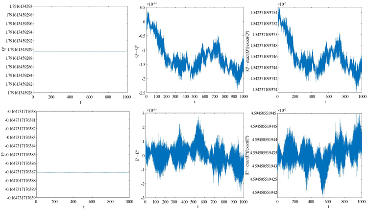
Figure 1. Total mass and energy and their difference from the initial values, and the corresponding relative errors of them in Example 1 ( $-a=b=50$, $T=1000$, $\alpha =0.2$, $\lambda =0.5$, ${\alpha }_1=1$, ${\alpha }_2=0$, $\beta =1$, $\gamma =0$, $\Gamma =0$, $h=1/8$, $\tau =1/64$ )

图1. 算例1离散下的总质量 $Q^k$ 和总能量 $E^k$，质量差 $Q^k-Q^0$ 和能量差 $E^k-E^0$，质量相对误差 $\left|Q^k-\text{real}\left(Q^0\right)\right|/\text{real}\left(Q^0\right)$ 和能量相对误差 $\left|E^k-\text{real}\left(E^0\right)\right|/\text{real}\left(E^0\right)$ ( $-a=b=50$, $T=1000$, $\alpha =0.2$, $\lambda =0.5$, ${\alpha }_1=1$, ${\alpha }_2=0$, $\beta =1$, $\gamma =0$, $\Gamma =0$, $h=1/8$, $\tau =1/64$ )

算例2

在如下初始值下 [5]

$u_0\left(x\right)=\sqrt{2}{r}_1\mathrm{sech}\left(r_{1}x+\frac{1}{2}{D}_0\right){\text{e}}^{i{V}_{0}x/4}$, $v_0\left(x\right)=\sqrt{2}{r}_2\mathrm{sech}\left(r_{2}x-\frac{1}{2}{D}_0\right){\text{e}}^{-i{V}_{0}x/4}$,

这里取 $-a=b=40$， $D_0=25$， $V_0=1$， ${\alpha }_1=1$， ${\alpha }_2=-\frac{1}{6}$， $\beta =1$， $\gamma =1$， $\Gamma =0.005$， $r_1=r_2=1$， $h=1/8$， $\tau =1/64$，用梯形积分公式 $\left(h=\tau =0.001\right)$ 算出原始微分方程组(1a~1d)的精确能量 $\text{real}\left(E^0\right)=5.083333333332668$ 和精确质量 $\text{real}\left(Q^0\right)=8$。

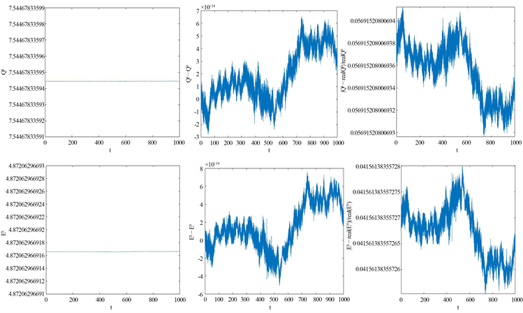
Figure 2. Total mass and energy and their difference from the initial values, and the corresponding relative errors of them in Example 2 ( $-a=b=40$, $T=1000$, $D_0=25$, $V_0=1$, ${\alpha }_1=1$, ${\alpha }_2=-\frac{1}{6}$, $\beta =1$, $\gamma =1$, $\Gamma =0.005$, $r_1=r_2=1$, $h=1/8$, $\tau =1/64$ )

图2. 算例2离散下的总质量 $Q^k$ 和总能量 $E^k$，质量差 $Q^k-Q^0$ 和能量差 $E^k-E^0$，质量相对误差 $\left|Q^k-\text{real}\left(Q^0\right)\right|/\text{real}\left(Q^0\right)$ 和能量相对误差 $\left|E^k-\text{real}\left(E^0\right)\right|/\text{real}\left(E^0\right)$ ( $-a=b=40$, $T=1000$, $D_0=25$, $V_0=1$, ${\alpha }_1=1$, ${\alpha }_2=-\frac{1}{6}$, $\beta =1$, $\gamma =1$, $\Gamma =0.005$, $r_1=r_2=1$, $h=1/8$, $\tau =1/64$ )

为了证实总质量和总能量在离散意义上的守恒，我们计算了离散下的能量和质量，数值能量和数值初始能量的差，以及数值能量与精确能量的相对误差。从图1和图2，我们可以看到，在离散意义下，总质量 $Q^k$ 和总能量 $E^k$ 随时间的变化总在一条直线上，说明随着时间t的计算，质量和能量是不变的，所以DFF格式很好地保持了总质量和总能量的守恒，验证了等式(8)和(9)中给出的守恒结果。因此，DFF格式满足守恒定律。

在测试线性耦合参数 $\Gamma$ 对两孤立波的碰撞影响，取定 $D_0=25$， $\beta =1$， ${\alpha }_1=1$， ${\alpha }_2=0$， $\gamma =0$， $V_0=1$， $r_1=r_2=1$。则只剩下自由参数 $\Gamma$。数值测试时， $\Gamma$ 分别取0.05，0.2，0.6，1。得出两种不同的孤立波在不同 $\Gamma$ 下的碰撞显示在图3中，同时 $\left|U^k\right|$ 和 $\left|V^k\right|$ 两个孤子在不同 $\Gamma$ 下的等高线图像显示在图4中。从这两幅图中可以看出，在不同 $\Gamma$ 下的碰撞是弹性的，原因是参数 ${\alpha }_2$ 被选取为0。此外，振幅在碰撞点有一些跳跃，这表明 $\left|U^k\right|$ 和 $\left|V^k\right|$ 之间发生了能量交换。并且线性耦合参数 $\Gamma$ 越大，跳跃越强。

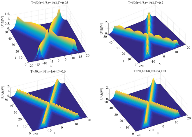
Figure 3. Elastic collision for Example 2 with ( $-a=b=20$, $T=50$, $D_0=25$, $V_0=1$, ${\alpha }_1=1$, ${\alpha }_2=0$, $\beta =1$, $\gamma =0$, $r_1=r_2=1$, $h=1/8$, $\tau =1/64$ )

图3. 算例2半弹性碰撞( $-a=b=20$, $T=50$, $D_0=25$, $V_0=1$, ${\alpha }_1=1$, ${\alpha }_2=0$, $\beta =1$, $\gamma =0$, $r_1=r_2=1$, $h=1/8$, $\tau =1/64$ )

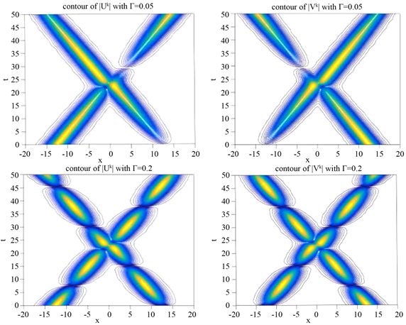
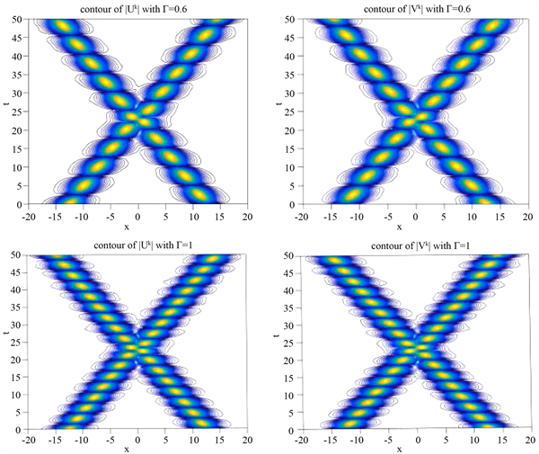
Figure 4. Evolution of the modulus of numerical solution for Example 2 with ( $-a=b=20$, $T=50$, $D_0=25$, $V_0=1$, ${\alpha }_1=1$, ${\alpha }_2=0$, $\beta =1$, $\gamma =0$, $r_1=r_2=1$, $h=1/8$, $\tau =1/64$ )

图4. 算例2数值解的模量演化( $-a=b=20$, $T=50$, $D_0=25$, $V_0=1$, ${\alpha }_1=1$, ${\alpha }_2=0$, $\beta =1$, $\gamma =0$, $r_1=r_2=1$, $h=1/8$, $\tau =1/64$ )

在测试非线性交叉项和初速度 $V_0$ 对两孤立波碰撞的影响时，取定 $\beta =1$， ${\alpha }_1=1$， $\gamma =0$， $\Gamma =0$， $r_1=1.2$， $r_2=1$，则剩下的自由参数为 ${\alpha }_2$ 和 $V_0$，初始位置参数 $D_0$ 可以任意选择。只要 $D_0$ 足够大，它们就不会影响碰撞结果。这里数值测试取 $D_0=25$。在测试中，取网格大小和时间步长为 $h=1/8$， $\tau =1/64$。

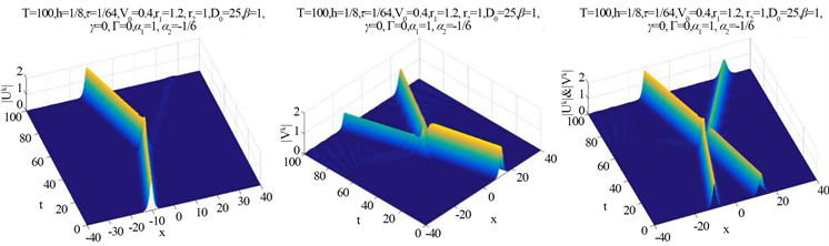
Figure 5. Evolution of the modulus of numerical solution for Example 2 with ( $-a=b=40$, $T=100$, $D_0=25$, $V_0=0.4$, ${\alpha }_1=1$, ${\alpha }_2=-1/6$, $\beta =1$, $\gamma =0$, $\Gamma =0$, $r_1=1.2$, $r_2=1$, $h=1/8$, $\tau =1/64$ )

图5. 算例2数值解的模量演化( $-a=b=40$, $T=100$, $D_0=25$, $V_0=0.4$, ${\alpha }_1=1$, ${\alpha }_2=-1/6$, $\beta =1$, $\gamma =0$, $\Gamma =0$, $r_1=1.2$, $r_2=1$, $h=1/8$, $\tau =1/64$ )

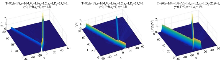
Figure 6. Evolution of the modulus of numerical solution for Example 2 with ( $-a=b=60$, $T=80$, $D_0=25$, $V_0=1.6$, ${\alpha }_1=1$, ${\alpha }_2=-1/6$, $\beta =1$, $\gamma =0$, $\Gamma =0$, $r_1=1.2$, $r_2=1$, $h=1/8$, $\tau =1/64$ )

图6. 算例2数值解的模量演化( $-a=b=60$, $T=80$, $D_0=25$, $V_0=1.6$, ${\alpha }_1=1$, ${\alpha }_2=-1/6$, $\beta =1$, $\gamma =0$, $\Gamma =0$, $r_1=1.2$, $r_2=1$, $h=1/8$, $\tau =1/64$ )

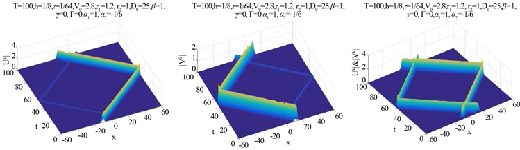
Figure 7. Evolution of the modulus of numerical solution for Example 2 with ( $-a=b=60$, $T=100$, $D_0=25$, $V_0=2.8$, ${\alpha }_1=1$, ${\alpha }_2=-1/6$, $\beta =1$, $\gamma =0$, $\Gamma =0$, $r_1=1.2$, $r_2=1$, $h=1/8$, $\tau =1/64$ )

图7. 算例2数值解的模量演化( $-a=b=60$, $T=100$, $D_0=25$, $V_0=2.8$, ${\alpha }_1=1$, ${\alpha }_2=-1/6$, $\beta =1$, $\gamma =0$, $\Gamma =0$, $r_1=1.2$, $r_2=1$, $h=1/8$, $\tau =1/64$ )

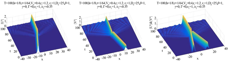
Figure 8. Evolution of the modulus of numerical solution for Example 2 with ( $-a=b=40$, $T=100$, $D_0=25$, $V_0=0.4$, ${\alpha }_1=1$, ${\alpha }_2=-0.35$, $\beta =1$, $\gamma =0$, $\Gamma =0$, $r_1=1.2$, $r_2=1$, $h=1/8$, $\tau =1/64$ )

图8. 算例2数值解的模量演化( $-a=b=40$, $T=100$, $D_0=25$, $V_0=0.4$, ${\alpha }_1=1$, ${\alpha }_2=-0.35$, $\beta =1$, $\gamma =0$, $\Gamma =0$, $r_1=1.2$, $r_2=1$, $h=1/8$, $\tau =1/64$ )

在第一种情况下，选择 ${\alpha }_2=-1/6$， $V_0=0.4$， $\beta =1$， ${\alpha }_1=1$， $\gamma =0$， $\Gamma =0$， $r_1=1.2$， $r_2=1$，结果如图5所示。从图中可以看出，右移的孤子被碰撞反射回来，也就是说，孤子的速度逐渐减小，当它从碰撞中出现时，速度变为负值。同样的事情也发生在左移孤子上。 [5] 中已经报告了这个反射场景。两个孤子的振幅在碰撞后也发生了变化，较大的孤子变得更大，较小的孤子变得更小。在这幅图中，我们还可以观察到一个小脉冲，它从孤立波中分离出来，沿着孤立波传播，这些波被称为子波。在第二种情况下，设置 ${\alpha }_2=-1/6$， $V_0=1.6$， $\beta =1$， ${\alpha }_1=1$， $\gamma =0$， $\Gamma =0$， $r_1=1.2$， $r_2=1$，如图6所示的结果。从这幅图中，我们可以观察到这两种波以某种重塑和辐射脱落的方式相互穿过，并产生子波。在第三种情况下，设置 ${\alpha }_2=-1/6$， $V_0=2.8$， $\beta =1$， ${\alpha }_1=1$， $\gamma =0$， $\Gamma =0$， $r_1=1.2$， $r_2=1$，并显示如图7所示的结果。从这幅图中，我们可以观察到这两种波相互穿过，且会彼此反弹并又相互穿过。在第四种情况下，我们设置 ${\alpha }_2=-0.35$， $V_0=0.4$， $\beta =1$， ${\alpha }_1=1$， $\gamma =0$， $\Gamma =0$， $r_1=1.2$， $r_2=1$，并显示如图8所示的结果。从图中可以观察到两个孤子融合为一个孤子，并产生一些小的子波。最后，设置 $r_1=1.4$ ${\alpha }_2=1$， $V_0=1.4$， $\beta =1$， $\gamma =0$， $\Gamma =0$， $r_1=1.2$， $r_2=1$，结果如图9所示。从这幅图中，我们可以观察到两个孤子碰撞后产生了新的孤子，同时也产生了一些小的子波。这些测试验证了 [27] 中给出的结果。

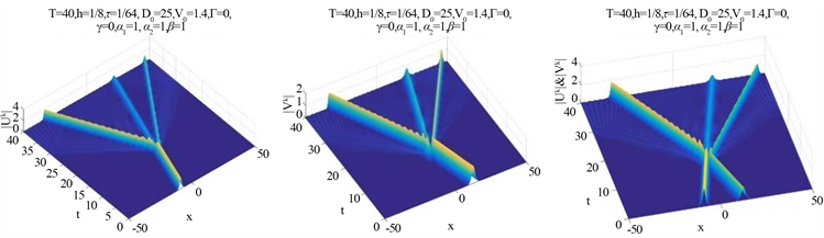
Figure 9. Evolution of the modulus of numerical solution for Example 2 with ( $-a=b=50$, $T=40$, $D_0=25$, $V_0=0.4$, ${\alpha }_1=1$, ${\alpha }_2=1$, $\beta =1$, $\gamma =0$, $\Gamma =0$, $r_1=1.4$, $r_2=1$, $h=1/8$, $\tau =1/64$ )

图9. 算例2数值解的模量演化( $-a=b=50$, $T=40$, $D_0=25$, $V_0=0.4$, ${\alpha }_1=1$, ${\alpha }_2=1$, $\beta =1$, $\gamma =0$, $\Gamma =0$, $r_1=1.4$, $r_2=1$, $h=1/8$, $\tau =1/64$ )

4. 结论

本文提出并分析了保结构Du Fort-Frankel有限差分法求解CNLS方程组。该格式大大缩短了系统的CPU时间。遗憾的是，该格式的收敛性没有给出，但在计算结果中可以发现，该格式是二阶的收敛精度。

基金项目

国家自然科学基金项目(No. 11861047)；江西省自然科学基金 (20202BABL201005)；江西省杰出青年基金 (20212ACB211006)。