基于Simulink的延迟微分方程框图求解

The Simulink-Based Box Diagram Solution to Delay Differential Equations

摘要: 微分方程是描述动态系统的最常用工具之一；延迟微分方程除包含有信号当前时刻的值外，还含有信号以前的值；若延迟微分方程只是复杂系统中的一部分，其输入信号来自于前一个模块，则无法用MATLAB编写匿名函数来直接求解；基于框图的仿真策略是解决这类问题的最好方法；Simulink是MATLAB下基于框图仿真方法的理想工具；用Simulink搭建延迟微分方程模型，并求出方程的数值解。

Abstract: Being one of the most commonly-used tools in describing the dynamic system, the delay differential equation contains not only the current value of the signal but also the previous one. However, it cannot be directly solved by writing anonymous functions with Matlab if the delay differential equation is only one part of the complex system, and its input signal comes from the previous module; therefore, the simulation strategy on the basis of the box diagram is the best way to solve such problems. Based on the box diagram, Matlab Simulink is the ideal tool, which helps build the delay differential equation model. By this way, we can solve the numerical solution of this equation.

1. 引言

微分方程是经济学、统计学、工程、科学计算等领域数学建模的基础，也常常被用来描述动态系统， $x^{\prime }\left(t\right)=f\left(t,x\left(t\right)\right)$ 是微分方程的一般形式，其全部信号都来自于时刻t的当前值。假若微分方程中既有时刻t的当前信号，也有早先时刻的信号值，这种微分方程就被称作延迟微分方程 [1] 。

2. 典型延迟微分方程的数值求解

延迟微分方程的一般形式为

$x^{\prime }\left(t\right)=f\left[t,x\left(t\right),x\left(t-{\xi }_1\right),x\left(t-{\xi }_2\right),\cdots ,x\left(t-{\xi }_n\right)\right],$

式中 ${\xi }_i$ 表示延迟常数，要求其为非负数且对应于 $x\left(t\right)$ 状态变量。与普通微分方程的差别在于，此处除了有当前时刻t的信号外，还有先前时刻的信号。因此延迟微分方程(组)的确定除必须有状态向量x和常规标量t外，还需设定 $\mathbb{Q}$ 矩阵， $\mathbb{Q}$ 中第j列的列向量 $\mathbb{Q}\left(:,j\right)$ 对应于延迟时间向量 ${\xi }_j$

例1设 $\{\begin{array}{l}4x\left(t\right)=2y\left(t\right)+3y^{\prime }\left(t\right)+y^{″}\left(t\right)\\ x^{\prime }\left(t\right)=0.2x^3\left(t-0.5\right)-x\left(t-0.5\right)-3x\left(t\right)-y\left(t-1\right)-1\end{array}$ ，

且当 $t\le 0$ 时 $x\left(t\right)=y\left(t\right)=y^{\prime }\left(t\right)=0$ ，试求解方程组。

解：方程组中包含了t， $t-1$ ， $t-0.5$ 时刻的信号值，故必须设计专门的算法和编写特定的程序来求解该延迟微分方程组，同时要转换成显式一阶方程组。引进一组状态变量 $x\left(t\right)=x_1\left(t\right),y\left(t\right)=x_2\left(t\right),y^{\prime }\left(t\right)=x_3\left(t\right)$ 是实现上述转换最便捷高效的方法。原方程组变形为：

$\{\begin{array}{l}{x^{\prime }}_3\left(t\right)=4x_1\left(t\right)-2x_2\left(t\right)-3x_3\left(t\right)\\ {x^{\prime }}_2\left(t\right)=x_3\left(t\right)\\ {x^{\prime }}_1\left(t\right)=0.2x_1^3\left(t-0.5\right)-x_1\left(t-0.5\right)-3x_1\left(t\right)-x_2\left(t-1\right)-1\end{array}$

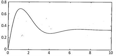
再引入时间常数 ${\xi }_1=1$ 对应状态变量 $x_2$ 、 ${\xi }_2=0.5$ 对应变量 $x_1$ ，用MATLAB编写匿名函数描述延迟微分方程，调用MATLAB语句使零向量对应常数初始值，在MATLAB运行程序即可得出该方程组的数值解 [2] ，如图1所示。

3. Simulink环境简介

假设一个系统能够用微分方程来进行描述，则使用前文介绍的求解函数就可以直接得出解。但如果微分方程仅仅是复杂系统中的一部分，输入信号本身由前一个模块传入，整个系统模型又无法用单独一个方程(组)来描述，这种情况下前面使用的求解函数则无能为力。

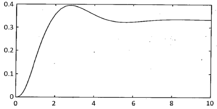(a) (b)

Figure 1. (a) The numerical solution of the delay differential equation (The initial condition is zero); (b) The numerical solution of the delay differential equation (The initial condition is non-zero)

图1. (a) 延迟微分方程的数值解(初始条件为零时)；(b) 延迟微分方程的数值解(初始条件为非零时)

解决这个问题的最有效途径就是仿真策略并基于框图实现。Matlab下的Simulink环境就是基于框图仿真策略的理想工具。

Math Works公司出品的Simulink，名字中Simu代表仿真，link表示连接，合起来的意思就是连接输入输出信号并且用框图来对某个系统进行仿真。求解微分方程(组)只是其众多的强大功能之一。

Simulink下支持的模块很多，如信号源输入模块组、自定义函数组等，如图2表示的常用模块组中可以自定义的模块组。

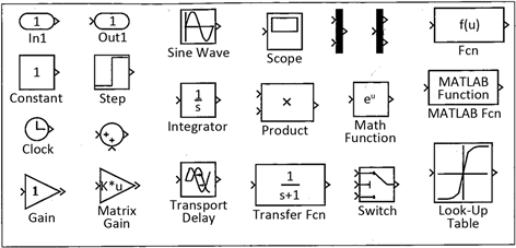
Figure 2. Commonly-used custom module groups

图2. 常用模块组中可以自定义的模块组

如图中Transport Delay表示延迟模块，本文正是用该模块来实现延迟微分方程的仿真建模与求解。

4. 延迟微分方程的Simulink建模

Simulink的Continuous组中提供了几个延迟模块，如图3所示，用于提取信号的延迟信息。

Figure 3. The Various delay modules provided by continuous function groups in Simulink

图3. Simulink的Continuous组提供的各种延迟模块

例如，Transport Delay模块描述的是传递函数 ${\text{e}}^{-Ls}$ ，L为延迟时间常数，若模块的输入信号为 $u\left(t\right)$ ，则其输出为 $u\left(t-L\right)$ ；若Variable Time Delay模块第二输入信号为t₀，则输出信号为 $u\left(t-t_0\right)$ ，而Variable Transport Delay模块是建立在Variable Time Delay模块基础上的可变传输延迟，第二端口为传输延迟t_i，由该值推算出一个等效的时间延迟t_d，则模块的输出信号为 $u\left(t-t_d\right)$ ，其中 ${\displaystyle {\int }_{t-t_d}^t\frac{1}{t_i\left(\xi \right)}\text{d}\xi }=1$ 。下面将通过例子演示框图构建与仿真方法。

例2考虑例1中的方程组，重写如下：

$\{\begin{array}{l}4x\left(t\right)=2y\left(t\right)+3y^{\prime }\left(t\right)+y^{″}\left(t\right)\\ x^{\prime }\left(t\right)=0.2x^3\left(t-0.5\right)-x\left(t-0.5\right)-3x\left(t\right)-y\left(t-1\right)-1\end{array}$

已知 $t\le 0$ 时 $x\left(t\right)=y\left(t\right)=y^{\prime }\left(t\right)=0$ ，用Simulink对该延迟微分方程组建模并仿真求解。

解：将方程式二中的 $-3x\left(t\right)$ 移到等式左边得

$3x\left(t\right)+x^{\prime }\left(t\right)=0.2x^3\left(t-0.5\right)-x\left(t-0.5\right)-y\left(t-1\right)-1$

表示在等号右边信号的激励下，x(t)传输函数模型 $1/\left(s+3\right)$ 的信号输出；另一个方程式表示在y(t)信号激励下，x(t)传递函数模块 $4/\left(s^2+3s+2\right)$ 的信号输出。

再在x(t)、y(t)上接入延迟模块Transport Delay，就可以生成这些信号的延迟。如此构建出如图4所示的Simulink仿真模型 [3] 。

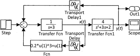
Figure 4. Simulink Modeling of the delay differential equation

图4. 延迟微分方程的Simulink建模

再调用语句

$>>\left[t,x\right]=sim\left(\text{'}c7mdde2\text{'},\left[0,10\right]\right)$ ；

$plot\left(t,x\right)$ ； %绘图显示仿真结果

得到与上文例1中图1(a)、图1(b)完全相同的曲线。

5. 延迟微分方程的Simulink模型仿真求解

例3已知延迟微分方程

$x^{\prime }\left(t\right)=M_1\cdot x\cdot \left(t-0.15\right)+M_2\cdot x^{\prime }\cdot \left(t-0.5\right)+K\cdot u\left(t\right),$

其中，输入信号 $u\left(t\right)\equiv 1$ ，且已知矩阵为

$M_1=\left[\begin{array}{ccc}-13& 3& -3\\ 106& -116& 62\\ 207& -207& 113\end{array}\right],M_2=\left[\begin{array}{ccc}0.02& 0& 0\\ 0& 0.03& 0\\ 0& 0& 0.04\end{array}\right],K=\left[\begin{array}{c}0\\ 1\\ 2\end{array}\right],$

试用Simulink搭建系统模型，并求出该方程的数值解。

解：因为方程中同时包含 $x^{\prime }\left(t\right)$ 和 $x^{\prime }\left(t-0.5\right)$ 项，所以单纯采用函数直接求解是无能为力的。可以采用Simulink仿真模型来求解。在构建框图前，在Matlab中先通过语句来生成已知矩阵，

$>>M1=\left[-13,3,-3;106,-116,62;207,-207,113\right];$

$M2=diag\left[0.02,0.03,0.04\right];$

$K=\left[0,1,2\right];$

因为状态向量 $x\left(t\right)$ 已经存在，只需添加一个积分器就可以构成输入端 $x^{\prime }\left(t\right)$ 、输出端 $x\left(t\right)$ ，之后给这两端信号接入延迟环节，设置适当的延迟时间常数，这样经过一系列处理就构建出如图5的Simulink框图模型。

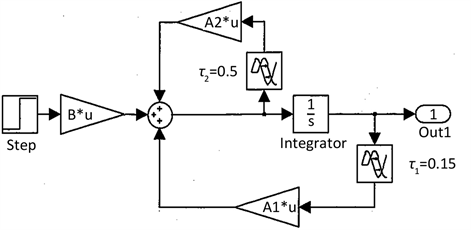
Figure 5. Simulink Modeling with the delay differential equation

图5. 带有导数延迟的微分方程的Simulink模型

再调用程序

$>>\left[t,x\right]=sim\left(\text{'}c7mdde3\text{'},\left[0,8\right]\right)$ ；

$plot\left(t,x\right)$ ； %将仿真结果绘图

得仿真解如图6所示 [4] 。

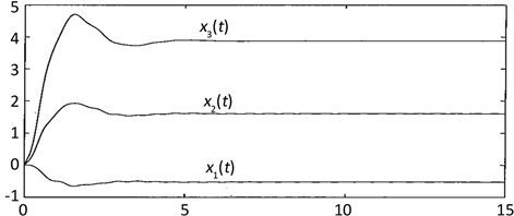
Figure 6. The Simulated experimental result of the delay differential equation

图6. 延迟微分方程的仿真实验结果

例4已知

$\{\begin{array}{l}{x^{\prime }}_1\left(t\right)=-2x_2\left(t\right)-3x_1\left(t-0.2\left|\sin t\right|\right)\\ {x^{\prime }}_2\left(t\right)=-0.05x_1\left(t\right)x_3\left(t\right)-2x_2\left(t-0.8\right)+2\\ {x^{\prime }}_3\left(t\right)=0.3x_1\left(t\right)x_2\left(t\right)x_3\left(t\right)+\cos \left[x_1\left(t\right)x_2\left(t\right)\right]+2\sin \left(0.1t^2\right)\end{array}$

各状态变量的初始条件均为零。试用仿真框图求解方程组。

解：要定义状态变量向量 $x\left(t\right)$ ，也需要添加一个向量型积分器，由信号

$x\left(t\right)$ ， $x_1\left(t-0.2\left|\sin t\right|\right)$ ， $x_2\left(t-0.8\right)$ ，t

等构成Mux模块的向量输出，得图7所示的仿真框图 [5] 。

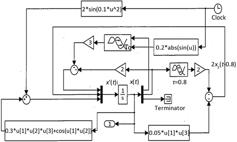
Figure 7. The Simulink model of the variable time delay differential equation

图7. 变时间延迟微分方程的 Simulink模型

图7中，使用Variable Time Delay模块实现变延迟时间， $0.2\cdot \left|\sin t\right|$ 代表第二路输入延迟，求得延迟微分方程的数值解如图8所示。

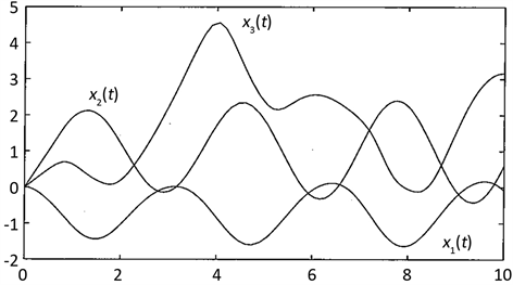
Figure 8. The simulated experimental numerical solution of the variable time delay differential equation

图8. 变时间延迟微分方程的仿真实验数值解