1. 介绍
对于固定的整数
,k重除数函数
是指
的解的个数,其中
为正整数。如果n的标准分解形式
,
(
),
(
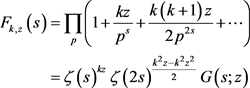
)是不同的素数,则有(可参见 [1] )
(1)
当
时,
即为经典除数函数
。
当
时,定义
的和函数
Landau [2] 和Voronoi [3] 证明了
其中
是
次的多项式。对于
,Hardy和Littlewood改进了以上余项的上界估计,证明了
相关文献还可参见 [4], [5], [6] 和 [7]。
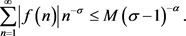
同时,人们还研究函数
在短区间上的均值问题。例如,Garaev,Luca和Nowak [8] 证明了当
时,有
当
时,目前短区间上相应问题的最佳结果可由
的渐进公式(“长区间”)推得。
本文中,我们考虑了
在短区间上另一种形式的均值问题。令
表示正整数n的不同素因子个数,定义
我们证明了下面的结果。
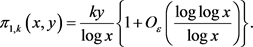
定理1.1对于固定的
,
及任意的
,有
对
,
,
一致成立,这里
并且O-符号中的隐含常数只依赖于B和
。
1939年,Erdös和Kac [9] 证明了
的概率分布,对于每一个
,他们证明了如下的中心极限定理:
其中
2015年,Elliott [10] [11] 证明了如下权为
(
)的中心极限定理,即对每一个
,有
其中
最近,K. Liu和J. Wu [12] 把此结果推广到了短区间。
本文中,我们推广了Elliott以及Liu和Wu的结果,证明了权为
的中心极限定理。
定理1.2对于每个实数
和任意的
,当
,
时,有
其中
O-符号中的隐含常数只依赖于
,并且误差项的上界估计是最优的。
记号:
N为全体自然数集,R为全体实数集,C为全体复数集;
伽马函数;Landau符号,
,
是指存在常数
,使得
;
表示p遍历所有素数并求乘积;
是指
。
2. 预备知识
为了完成引理2.2的证明,我们需要下面的定义(参见 [12] )。令
表示算术函数,
是
的Dirichlet级数,
设
,
,
,
,
,
,
,
为常数,
。如果
满足下列条件,则称其是
型的:
(a) 对于任意的
,有
-中的隐含常数只与
有关。
(b) 当
时有
(c) Dirichlet级数

可以解析延拓成 上的全纯函数,并且
 满足
满足

此结果对 ,
, 及
及 一致成立。
一致成立。
我们需要如下引理来证明引理2.2,此引理为 [1] 的推论1.2。
引理2.1假设对任意的 ,Dirichlet级数
 是
是 型的,则有
型的,则有
此结果对 ,
, ,
, ,及
,及 一致成立,其中

O-符号中的隐含常数只依赖于A,B, ,
, 及
及 。
。
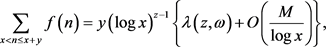
令引理2.1中的 ,我们得到如下结果。
引理2.2令 是一个常数,对于任意的
 ,有
,有

对 ,
, ,及
,及 一致成立,其中
证明:因为函数 是可乘函数,当
 时,我们有
时,我们有
 (2)
(2)
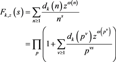
把公式(1)带入公式(2)中,可得
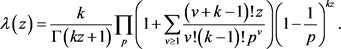
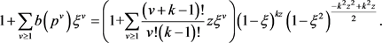
其中欧拉乘积

 的Dirichlet级数是

令 ,当
,当 时,函数
时,函数 是可乘函数,其在
 (p为素数,
 )的值可由下列公式给出
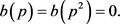
特别地,当 ,
, 时,对于所有的素数p有
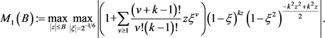
令

因为当 ,
, 时函数
时函数 收敛,所以该函数在
 ,
, 时有最大值:
由Cauchy公式,当 ,
, 时有
时有

所以 的上界为
的上界为
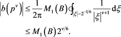 (3)
(3)
当 ,
, 时,计算可得

再由公式(3)可得
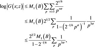
这表明 在
在 ,
, 时收敛,且
时收敛,且 有上界:
有上界:

其中
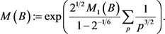
综合上述计算结果,我们可以得到Dirichlet级数 是
是
 型的。
型的。
这样应用引理2.1我们可以得到引理2.2. □
注记:如果 ,则由引理2.2可以推出

对 ,
, 一致成立,其中

在证明定理1.2时,我们还需要下面的Berry-Esseen不等式(可参见 [13] )。
引理2.3令F、G为两个分布函数,f、g分别为F、G的特征函数。假设G可导,且 在R上有界。则有

对所有的 都成立。其中
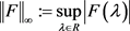 。
。
3. 定理1.1的证明
设
由Cauchy公式,可得
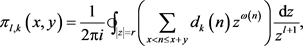
其中 。
。
由引理2.2,可得
 (4)
(4)
其中

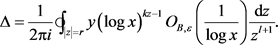
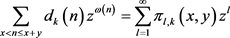
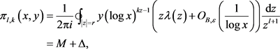
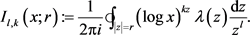
首先计算 的主项M,令
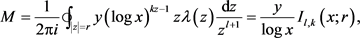
其中
接下来计算 ,考虑
,考虑 和
和 两种情况。当
 时,因为
时,因为 在
在 时解,所以
时解,所以

将此结果代入公式(4),得到
当 时,因为
时,因为 在
在 时解析,所以
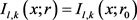 ,其中
,其中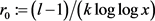 。
。 在点
在点 处的Taylor展开为
 (5)
(5)
这样,我们只需分别估计上述公式(5)右侧的三项对 的贡献即可。
第一项对 的贡献为:
的贡献为:
 (6)
(6)
第二项对 的贡献为:
的贡献为:
 (7)
(7)
当 ,
, ,
, 时,有
时,有

因为当 时
时 解析,所以
解析,所以 在
在 上有上界,即存在一个常数
 ,使得
,使得 ,容易计算出

由Stirling公式,第三项对 的贡献为:
的贡献为:
 (8)
(8)
现在来估计 的余项
的余项 。我们有
。我们有

令 ,可得
,可得

将公式(6) (7)、(8)代入公式(4),即得定理1.1。
4. 定理1.2的证明
令 ,记
,记 为
为 的特征函数,我们有
 (9)
(9)
其中 。
。
设 ,由引理2.3,计算得到下面结果:

所以我们只需要证明
 (10)
(10)
对 ,
, 时一致成立。
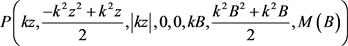
由引理2.2,设 ,则有
,则有

对 ,
, ,
, 一致成立,其中
 是关于z的整数函数,且
 。令
。令 ,则有
,则有

对 ,
, 及
及 一致成立。
一致成立。
当 时,因为
时,因为 ,所以有
,所以有

由此可以推出 对
对 ,
, 及
及 一致成立。下面我们将分三种情况来证明公式(10)成立。
首先,当 时,有
时,有
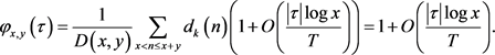
其次,当 时,因为
时,因为

则有
将上式代入公式(9),得到
由此可得,

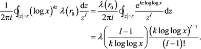
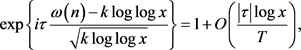
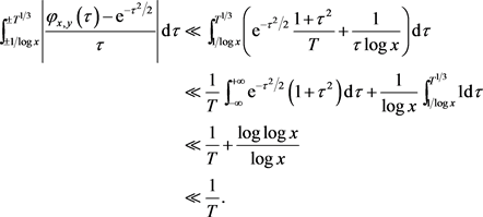
最后,当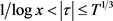 时,由
时,由 和
和 的Taylor展开:

可得

对 ,
, ,
, 一致成立。计算可得
现在我们来证明定理1.2中的余项估计是最优的。定义
以及
令 ,
, ,我们得到
,我们得到
 (11)
(11)
由Stirling公式及定理1.1,可得
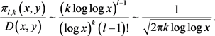 (12)
(12)
根据公式(11)及公式(12),可以求得
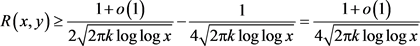
对 ,
, 一致成立。由此可见,定理1.2中的余项估计是最优的。