基于不动点理论的分数阶模糊细胞神经网络的稳定性分析

doi:10.12677/PM.2024.143082

期刊菜单

基于不动点理论的分数阶模糊细胞神经网络的稳定性分析
Stability Analysis of Fractional Order Fuzzy Cellular Neural Networks via Fixed Point Approach

DOI: 10.12677/PM.2024.143082, PDF, HTML, XML, 下载: 36 浏览: 109 科研立项经费支持
作者: 熊希曦, 罗敏：云南财经大学统计与数学学院，云南昆明；陈龙伟^*：云南财经大学云南省服务计算重点实验室，云南昆明；云南财经大学智能应用研究院，云南昆明
关键词: 分数阶神经网络；压缩映射理论；全局指数稳定性；Fractional Order Neural Networks； Contraction Mapping Theory； Global Exponential Stability

摘要: 针对具有时变时滞的分数阶模糊细胞神经网络，采用Banach不动点理论和方法，直接得到了分数阶神经网络的一个新的稳定性判据。该方法较为新颖，得到比已有结果更简单的结论。最后，给出了一个数值例子来说明所提方法的有效性。

Abstract: For fractional-order fuzzy cellular neural networks with time-varying delays, Banach fixed point theory and technique are employed to derive a new stability criterion of fractional-order neural networks. This method is relatively novel, and a simpler conclusion is obtained than the existing results. Finally, a numerical example is given to illustrate the effectiveness of the proposed method.

文章引用：熊希曦, 陈龙伟, 罗敏. 基于不动点理论的分数阶模糊细胞神经网络的稳定性分析[J]. 理论数学, 2024, 14(3): 19-31. https://doi.org/10.12677/PM.2024.143082

1. 引言

近年来，许多研究者提出并研究了细胞神经网络(CNN) [1] [2] 。到目前为止，已经提出了三种基本的细胞神经网络(CNN)结构。第一个是传统的CNN [3] ；第二种是延迟型CNN [4] ；最后一个是离散时间CNN [5] 。与传统的CNN结构不同，模糊细胞神经网络(FCNN)除了产品运算的总和外，还在其模板输入和/或输出之间实现了模糊逻辑。与细胞神经网络不同，模糊细胞神经网络将模糊逻辑集成到传统细胞神经系统的结构中，并保持细胞之间的邻近连接。模糊细胞神经网络(FCNNs)，由Yang等人 [6] 提出，并具有广泛应用，如思维和推理、白细胞检测和模式识别 [7] [8] [9] 。

神经网络模型的设计和实际适用性在很大程度上取决于其稳定性特性。与传统CNN类似，系统的稳定性在FCNN的设计中非常重要，前人已经提出了FCNN的几个条件 [10] [11] [12] 。分数阶神经网络在时序预测、图像处理、自然语言处理方面 [13] [14] [15] 有重要应用。稳定性是不同类别的分数阶模型中研究最多的定性之一，包括分数阶神经网络模型，现已有很多研究分数阶神经网络的解的存在唯一性和稳定性分析，但基本使用的是Lyapunov函数方法 [16] - [21] 。然而，使用不动点理论直接得出稳定性的，基本是对于整数阶神经网络 [22] [23] [24] 。

因此，本文应用不动点理论研究了分数阶模糊细胞神经网络的全局指数稳定性问题。利用Caputo分数阶积分导数等定义进行计算，在乘积空间上构造映射，并证明了这个映射是连续的、自射的、压缩的，从而直接得到了该系统解的稳定性判据。方法不同，应用对象不同，结论也就不同于以往文献。

2. 预备知识

模型是在n维欧式空间 $R^{n}$ 中， $Ω$ 有界开集，光滑边界 $\partial Ω$ ，测度 $m e s Ω > 0$ 。考虑下列分数阶模糊细胞神经网络系统

$\begin{matrix} {}_{Ω}^{C}D_{t}^{α} w_{i} (t, x) = - c_{i} w_{i} (t, x) + \sum_{j = 1}^{m} a_{i j} g_{j} (w_{j} (t, x)) + \sum_{j = 1}^{m} b_{i j} g_{j} (w_{j} (t - τ_{j} (t), x)) + I_{i} \\ + \sum_{j = 1}^{m} h_{i j} μ_{j} + \land_{j = 1}^{m} u_{i j} g_{j} (w_{j} (t - τ_{j} (t), x)) + \land_{j = 1}^{m} R_{i j} μ_{j} + \lor_{j = 1}^{m} v_{i j} g_{j} (w_{j} (t - τ_{j} (t), x)) + \lor_{j = 1}^{m} Q_{i j} μ \end{matrix}$ (1)

狄利克雷(Dirichlet)边界和初始条件：

$w_{i} (s, x) = ξ_{i} (s, x), s \in [- τ, 0], x \in Ω_{j}$ (2)

$w_{i} (t, x) = 0, t \in [- τ, \infty), x \in \partial Ω$

其中， $t > 0$ ， $i = 1, 2, \dots, n$ ， $n \geq 2$ ，对应于神经网络中的单元数； $w = {(w_{1}, w_{2} \dots, w_{n})}^{T} \in R^{n}$ ， $w_{i} (t, x)$ 对应于第i个单元在时间t和空间x的状态； $g_{j} (w_{j})$ 表示第j个单元的激活函数。进一步地， $a_{i j}, b_{i j}, I_{i}, c_{i}$ 是常数； $a_{i j}$ 表示在时间t和空间x中第i个单元上第j个单元的强度； $b_{i j}$ 表示在时间 $t - τ_{j} (t)$ 和空间x中第i个单元上第j个单元的强度； $I_{i}$ 表示第i个单元上的外部偏置， $c_{i}$ 表示当与网络和外部输入断开连接时，第i个单元将其电位重置为隔离状态的速率。此外， $τ_{j} (t)$ 对应于沿第j个单元的轴突的传输延迟。 $h_{i j}$ 是前馈模板的元素。 $u_{i j}, v_{i j}, R_{i j}, Q_{i j}$ 分别是模糊反馈最小模板、模糊反馈最大模板的元素。 $\land$ 和 $\lor$ 分别表示模

糊或运算和模糊和运算。

注1：虽然文献 [18] 中也应用了Banach不动点定理，但本文所用的方法与文献 [18] 不同，我们直接用Banach不动点定理导出了稳定性判据。

定义1 [25] 对于任意 $t > 0$ ，函数 $l \in C^{1} [[0, b] \times Ω, R], b > 0$ ， $0 < α < 1$ 的下限为0，则 $α$ 阶的时间Caputo分数阶导数定义为：

${}_{0}^{C}D_{t}^{α} l (t, x) = \frac{1}{Γ (1 - α)} \int_{0}^{t} \frac{\partial l (s, x)}{\partial s} \frac{d s}{{(t - s)}^{α}} .$

$Γ$ 是伽马函数。

定义2 [24] 对于任意的初始条件 $(ξ (s)) \in C ([- τ, 0], R^{n + m})$ ，系统(1)和(2)被称为全局指数稳定的，如果存在 $a > 0, b > 0$ 使得

$‖ (w (t; s, ξ)) ‖ \leq b e^{- a t}, t > 0$

定义的范数为 $‖ w (t) ‖ = {(\sum_{i = 1}^{n} {| w_{i} (t) |}^{2})}^{1 / 2}$ ， $ξ = {(ξ_{1}, \dots, ξ_{n})}^{T}$ ， $w = {(w_{1}, \dots, w_{n})}^{T}$ 。

引理1 [26] 设区间 $[0, t]$ 被分为M份，记为 $0 = t_{0} < t_{1} < \dots < t_{M} = t$ ， $Δ t_{i} = t_{i} - t_{i - 1}$ ， $i = 1, \dots, M$ ，于是有

${}_{0}^{C}D_{t}^{α} w (t_{M}) = \frac{1}{Γ (2 - α)} \sum_{i = 1}^{M} d_{i} w (t_{i}) .$

其中， $i = 0$ 时， $d_{0} = \frac{t_{M}^{1 - α} - {(t_{M} - t_{1})}^{1 - α}}{t_{1}}$ ； $i \in (1, M - 1)$ 时， $d_{i} = \frac{{(t_{M} - t_{i - 1})}^{1 - α} - {(t_{M} - t_{i})}^{1 - α}}{Δ t_{i}} - \frac{{(t_{M} - t_{i})}^{1 - α} - {(t_{M} - t_{i + 1})}^{1 - α}}{Δ t_{i + 1}}$ ； $i = M$ 时， $d_{M} = \frac{{(t_{M} - t_{M - 1})}^{1 - α}}{t_{M} - t_{M - 1}}$ 。

引理2 [6] x与 $x^{'}$ 是模糊细胞神经网络的两种状态，于是我们有

$| \land_{j = 1}^{m n} u_{i j} f_{j} (x_{j}) - \land_{j = 1}^{m n} u_{i j} f_{j} ({x^{'}}_{j}) | \leq \sum_{j = 1}^{m n} | u_{i j} | | f_{j} (x_{j}) - f_{j} ({x^{'}}_{j}) |$ ;

$| \lor_{j = 1}^{m n} u_{i j} f_{j} (x_{j}) - \lor_{j = 1}^{m n} u_{i j} f_{j} ({x^{'}}_{j}) | \leq \sum_{j = 1}^{m n} | u_{i j} | | f_{j} (x_{j}) - f_{j} ({x^{'}}_{j}) |$ .

为了确保接下来的计算和证明，我们提出了以下假设：

1. (Lipschitz连续)激活函数 $g_{j}$ 是Lipschitz连续的，如果存在常数 $L_{j} > 0 (j = 1, 2, \dots, m)$ 使得

$| g_{j} (z) - g_{j} (w) | \leq L_{j} | z - w |$

并且有 $g_{j} (0) = 0$ ， $z, w \in R$ ， $z \neq w$ 。

3. 主要结果

在本节中，我们假设 $δ$ 是一个足够小的正数，并且假设1成立。

定理1 系统(1)和(2)是全局指数稳定的，如果存在一个正标量 $κ < 1$

$κ = \max_{i \in Ν} {| \frac{1}{Γ (α)} | \cdot [c_{i} + \sum_{j = 1}^{m} (| a_{i j} | + | b_{i j} | + | u_{i j} | + | v_{i j} |) L_{j}]} .$ (3)

证明：所有的证明可以分为四个步骤：

第一步，首先要构造映射即需要构造一个算子，那么根据引理1以及指数函数一些性质，我们需要对于Caputo分数阶导数利用线性插值进行形式变换，将指数函数代入构造所需算子。

$\begin{matrix} {}_{0}^{C}D_{t}^{α} (e^{t} \cdot w (t)) = \frac{1}{Γ (1 - α)} \int_{0}^{t} \frac{\partial (e^{s} \cdot w (s))}{\partial s} \frac{d s}{{(t - s)}^{α}} = \frac{1}{Γ (1 - α)} \sum_{i = 1}^{M} d_{i} e^{t_{i}} w (t_{i}) \\ \leq e^{t} \frac{1}{Γ (1 - α)} \sum_{i = 1}^{M} d_{i} w (t_{i}) = e^{t} {}_{0}^{C}D_{t}^{α} w (t) \\ = e^{t} [- c_{i} w_{i} (t, x) + \sum_{j = 1}^{m} a_{i j} g_{j} (w_{j} (t, x)) + \sum_{j = 1}^{m} b_{i j} g_{j} (w_{j} (t - τ_{j} (t), x)) \\ + \sum_{j = 1}^{m} h_{i j} μ_{j} + \land_{j = 1}^{m} u_{i j} g_{j} (w_{j} (t - τ_{j} (t), x)) + I_{i} \\ + \land_{j = 1}^{m} R_{i j} μ_{j} + \lor_{j = 1}^{m} v_{i j} g_{j} (w_{j} (t - τ_{j} (t), x)) + \lor_{j = 1}^{m} Q_{i j} μ_{j}] \end{matrix}$

则 ${}_{Ω}^{C}D_{t}^{α} (e^{t} \cdot w (t))$ 取上界，再两边同时分数阶积分

$e^{t} \cdot w_{i} (t) - ξ_{i} (0) = J^{α} [e^{t} \cdot {}_{Ω}^{C}D_{t}^{α} w_{i} (t)]$

$w_{i} (t) = e^{- t} \cdot {ξ_{i} (0) + J^{α} [e^{t} \cdot {}_{Ω}^{C}D_{t}^{α} w_{i} (t)]}$

从而，我们就构造了一个算子 $Θ$ ， $Θ = (Θ_{1}, Θ_{2}, Θ_{3}, \dots, Θ_{n})$ ， $Θ_{i} : χ_{i} \to χ_{i}$ 如下：

${\begin{array}{l} Θ_{i} w_{i} (t, x) = e^{- t} \cdot {ξ_{i} (0) + \frac{1}{Γ (α)} \int_{0}^{t} e^{t} {(t - s)}^{α - 1} \cdot [- c_{i} w_{i} (s, x) + \sum_{j = 1}^{m} a_{i j} g_{j} (w_{j} (s, x)) \\ + \sum_{j = 1}^{m} b_{i j} g_{j} (w_{j} (s - τ_{j} (s), x)) + I_{i} + \sum_{j = 1}^{m} h_{i j} μ_{j} + \land_{j = 1}^{m} u_{i j} g_{j} (w_{j} (s - τ_{j} (s), x)) + \land_{j = 1}^{m} R_{i j} μ_{j} \\ + \lor_{j = 1}^{m} v_{i j} g_{j} (w_{j} (s - τ_{j} (s), x)) + \lor_{j = 1}^{m} Q_{i j} μ_{j}] d s}, t \geq 0, i \in Ν \\ Θ_{i} w_{i} (s, x) = ξ_{i} (s, x), s \in [- τ, 0], x \in Ω \\ Θ_{i} w_{i} (t, x) = 0, s \in [- τ, \infty], x \in \partial Ω \end{array}$ (4)

定义的距离为：

$d i s t (w, z) = \max_{i \in Ν} (\sup_{t \geq - τ} | w_{i} (t, x) - z_{i} (t, x) |), \forall w, z \in χ_{1} \times χ_{2} \times \dots \times χ_{n}$ (5)

可见， $χ_{1} \times χ_{2} \times \dots \times χ_{n}$ 是一个完备的度量空间。

第二步，要证明(4)对于 $t \in [0, + \infty)$ 上是连续的，那么令 $δ$ 是足够小的标量。

$\begin{array}{l} | Θ_{i} w_{i} (t + δ, x) - Θ_{i} w_{i} (t, x) | \\ = | e^{- (t + δ)} \cdot {ξ_{i} (0, x) + \frac{1}{Γ (α)} \int_{0}^{t + δ} e^{s} {(t - s)}^{α - 1} \cdot [- c_{i} w_{i} (s, x) + \sum_{j = 1}^{m} a_{i j} g_{j} (w_{j} (s, x)) \\ + \sum_{j = 1}^{m} b_{i j} g_{j} (w_{j} (s - τ_{j} (s), x)) + I_{i} + \sum_{j = 1}^{m} h_{i j} μ_{j} + \land_{j = 1}^{m} u_{i j} g_{j} (w_{j} (s - τ_{j} (s), x)) + \land_{j = 1}^{m} R_{i j} μ_{j} \\ + \lor_{j = 1}^{m} v_{i j} g_{j} (w_{j} (s - τ_{j} (s), x)) + \lor_{j = 1}^{m} Q_{i j} μ_{j}] d s} \end{array}$

$\begin{array}{l} - e_{i}^{- t} \cdot {ξ_{i} (0, x) + \frac{1}{Γ (α)} \int_{0}^{t} e_{i}^{s} {(t - s)}^{α - 1} \cdot [- c_{i} w_{i} (s, x) + \sum_{j = 1}^{m} a_{i j} g_{j} (w_{j} (s, x)) \\ + \sum_{j = 1}^{m} b_{i j} g_{j} (w_{j} (s - τ_{j} (s), x)) + I_{i} + \sum_{j = 1}^{m} h_{i j} μ_{j} + \land_{j = 1}^{m} u_{i j} g_{j} (w_{j} (s - τ_{j} (s), x)) + \land_{j = 1}^{m} R_{i j} μ_{j} \\ + \lor_{j = 1}^{m} v_{i j} g_{j} (w_{j} (s - τ_{j} (s), x)) + \lor_{j = 1}^{m} Q_{i j} μ_{j}] d s} | \end{array}$

$\begin{array}{l} \leq | e^{- (t + δ)} \cdot ξ_{i} (0, x) - e_{}^{- t} \cdot ξ_{i} (0, x) | + | \frac{e^{- (t + δ)}}{Γ (α)} \int_{0}^{t + δ} e^{s} {(t - s)}^{α - 1} \cdot [- c_{i} w_{i} (s, x) + \sum_{j = 1}^{m} a_{i j} g_{j} (w_{j} (s, x)) \\ + \sum_{j = 1}^{m} b_{i j} g_{j} (w_{j} (s - τ_{j} (s), x)) + I_{i} + \sum_{j = 1}^{m} h_{i j} μ_{j} + \land_{j = 1}^{m} u_{i j} g_{j} (w_{j} (s - τ_{j} (s), x)) + \land_{j = 1}^{m} R_{i j} μ_{j} \\ + \lor_{j = 1}^{m} v_{i j} g_{j} (w_{j} (s - τ_{j} (s), x)) + \lor_{j = 1}^{m} Q_{i j} μ_{j}] d s - \frac{e_{i}^{- t}}{Γ (α)} \int_{0}^{t} e_{i}^{s} {(t - s)}^{α - 1} \cdot [- c_{i} w_{i} (s, x) + \sum_{j = 1}^{m} a_{i j} g_{j} (w_{j} (s, x)) \\ + \sum_{j = 1}^{m} b_{i j} g_{j} (w_{j} (s - τ_{j} (s), x)) + I_{i} + \sum_{j = 1}^{m} h_{i j} μ_{j} + \land_{j = 1}^{m} u_{i j} g_{j} (w_{j} (s - τ_{j} (s), x)) + \land_{j = 1}^{m} R_{i j} μ_{j} \\ + \lor_{j = 1}^{m} v_{i j} g_{j} (w_{j} (s - τ_{j} (s), x)) + \lor_{j = 1}^{m} Q_{i j} μ_{j}] d s | \end{array}$

将上式不等号右边分成以下两式分别求解：

显然有

$| e^{- (t + δ)} \cdot ξ_{i} (0, x) - e^{- t} \cdot ξ_{i} (0, x) | = | [e^{- (t + δ)} - e^{- t}] \cdot ξ_{i} (0, x) | \to 0, δ \to 0;$

接下来可得：

$\begin{array}{l} | \frac{e^{- (t + δ)}}{Γ (α)} \int_{0}^{t + δ} e^{s} {(t - s)}^{α - 1} \cdot [- c_{i} w_{i} (s, x) + \sum_{j = 1}^{m} a_{i j} g_{j} (w_{j} (s, x)) + \sum_{j = 1}^{m} b_{i j} g_{j} (w_{j} (s - τ_{j} (t), x)) + I_{i} \\ + \sum_{j = 1}^{m} h_{i j} μ_{j} + \land_{j = 1}^{m} u_{i j} g_{j} (w_{j} (s - τ_{j} (s), x)) + \land_{j = 1}^{m} R_{i j} μ_{j} + \lor_{j = 1}^{m} v_{i j} g_{j} (w_{j} (s - τ_{j} (s), x)) + \lor_{j = 1}^{m} Q_{i j} μ_{j}] d s \\ - \frac{e^{- t}}{Γ (α)} \int_{0}^{t} e^{s} {(t - s)}^{α - 1} \cdot [- c_{i} w_{i} (s, x) + \sum_{j = 1}^{m} a_{i j} g_{j} (w_{j} (s, x)) + \sum_{j = 1}^{m} b_{i j} g_{j} (w_{j} (s - τ_{j} (s), x)) + I_{i} \\ + \sum_{j = 1}^{m} h_{i j} μ_{j} + \land_{j = 1}^{m} u_{i j} g_{j} (w_{j} (s - τ_{j} (s), x)) + \land_{j = 1}^{m} R_{i j} μ_{j} + \lor_{j = 1}^{m} v_{i j} g_{j} (w_{j} (s - τ_{j} (s), x)) + \lor_{j = 1}^{m} Q_{i j} μ_{j}] d s | \end{array}$

$\begin{array}{l} \leq | \frac{e^{- (t + δ)}}{Γ (α)} \int_{t}^{t + δ} e^{ϖ_{i} (s)} {(t - s)}^{α - 1} \cdot [- c_{i} w_{i} (s, x) + \sum_{j = 1}^{m} a_{i j} g_{j} (w_{j} (s, x)) + \sum_{j = 1}^{m} b_{i j} g_{j} (w_{j} (s - τ_{j} (t), x)) + I_{i} \\ + \sum_{j = 1}^{m} h_{i j} μ_{j} + \land_{j = 1}^{m} u_{i j} g_{j} (w_{j} (s - τ_{j} (s), x)) + \land_{j = 1}^{m} R_{i j} μ_{j} + \lor_{j = 1}^{m} v_{i j} g_{j} (w_{j} (s - τ_{j} (s), x)) + \lor_{j = 1}^{m} Q_{i j} μ_{j}] d s | \\ + | (\frac{e_{i}^{- (t + δ)}}{Γ (α)} - \frac{e_{i}^{- t}}{Γ (α)}) \int_{0}^{t} e_{i}^{s} {(t - s)}^{α - 1} \cdot [- c_{i} w_{i} (s, x) + \sum_{j = 1}^{m} a_{i j} g_{j} (w_{j} (s, x)) + \sum_{j = 1}^{m} b_{i j} g_{j} (w_{j} (s - τ_{j} (s), x)) + I_{i} \\ + \sum_{j = 1}^{m} h_{i j} μ_{j} + \land_{j = 1}^{m} u_{i j} g_{j} (w_{j} (s - τ_{j} (s), x)) + \land_{j = 1}^{m} R_{i j} μ_{j} + \lor_{j = 1}^{m} v_{i j} g_{j} (w_{j} (s - τ_{j} (s), x)) + \lor_{j = 1}^{m} Q_{i j} μ_{j}] d s | \to 0, δ \to 0; \end{array}$

因此，证明了系统在 $t \in [0, + \infty)$ 上是连续的。

第三步，要证明 $| e^{γ t} Θ_{i} w_{i} (t, x) | \to 0, t \to + \infty, γ \in (0, 1)$ ，基于 $| e^{γ \begin{matrix} t \end{matrix}} X_{i} (t, x) | \to 0$ ，有 $| e^{γ \begin{matrix} t \end{matrix}} X_{i} (t, x) {(Δ t)}^{α - 1} | \to 0$ ， $Δ t = t - s$ ， $s \in [0, t]$ ，则 $\forall ε > 0, t^{*} \geq τ$ 使得 $| e^{γ \begin{matrix} t \end{matrix}} X_{i} (t, x) {(Δ t)}^{α - 1} | < ε μ, t \geq t^{*}, μ = {(1, 1, \dots, 1)}^{T}$ 。

$\begin{array}{l} | e^{γ \begin{matrix} t \end{matrix}} Θ_{i} w_{i} (t, x) | \\ = e^{γ \begin{matrix} t \end{matrix}} \cdot | e^{- t} \cdot {ξ_{i} (0, x) + \frac{1}{Γ (α)} \int_{0}^{t} e^{s} {(t - s)}^{α - 1} \cdot [- c_{i} w_{i} (s, x) + \sum_{j = 1}^{m} a_{i j} g_{j} (w_{j} (s, x)) \\ + \sum_{j = 1}^{m} b_{i j} g_{j} (w_{j} (s - τ_{j} (t), x)) + I_{i} + \sum_{j = 1}^{m} h_{i j} μ_{j} + \land_{j = 1}^{m} u_{i j} g_{j} (w_{j} (s - τ_{j} (s), x)) \\ + \land_{j = 1}^{m} R_{i j} μ_{j} + \lor_{j = 1}^{m} v_{i j} g_{j} (w_{j} (s - τ_{j} (t), x)) + \lor_{j = 1}^{m} Q_{i j} μ_{j}] d s} | \end{array}$

$\begin{array}{l} \leq e^{γ \begin{matrix} t \end{matrix}} | e_{i}^{- t} \cdot ξ_{i} (0, x) | + e^{γ \begin{matrix} t \end{matrix}} | \frac{e^{- t}}{Γ (α)} \int_{0}^{t} e^{s} {(t - s)}^{α - 1} \cdot (- c_{i} w_{i} (s, x)) d s | \\ + e^{γ \begin{matrix} t \end{matrix}} | \frac{e^{- t}}{Γ (α)} \int_{0}^{t} e^{s} {(t - s)}^{α - 1} \cdot \sum_{j = 1}^{m} a_{i j} g_{j} (w_{j} (s, x)) d s | \\ + e^{γ \begin{matrix} t \end{matrix}} | \frac{e^{- t}}{Γ (α)} \int_{0}^{t} e^{s} {(t - s)}^{α - 1} \cdot \sum_{j = 1}^{m} b_{i j} g_{j} (w_{j} (s - τ_{j} (s), x)) d s | \\ + e^{γ \begin{matrix} t \end{matrix}} | \frac{e^{- t}}{Γ (α)} \int_{0}^{t} e^{s} {(t - s)}^{α - 1} \cdot [I_{i} + \sum_{j = 1}^{m} h_{i j} μ_{j} + \land_{j = 1}^{m} R_{i j} μ_{j} + \lor_{j = 1}^{m} Q_{i j} μ_{j}] d s | \\ + e^{γ \begin{matrix} t \end{matrix}} | \frac{e^{- t}}{Γ (α)} \int_{0}^{t} e^{s} {(t - s)}^{α - 1} \cdot [\land_{j = 1}^{m} u_{i j} g_{j} (w_{j} (s - τ_{j} (s), x))] d s | \\ + e^{γ \begin{matrix} t \end{matrix}} | \frac{e^{- t}}{Γ (α)} \int_{0}^{t} e^{s} {(t - s)}^{α - 1} \cdot [\lor_{j = 1}^{m} v_{i j} g_{j} (w_{j} (s - τ_{j} (s), x))] d s | \end{array}$

将上式分成以下分式，具体计算过程如下：

显然地，有

$e^{γ \begin{matrix} t \end{matrix}} | e^{- t} \cdot ξ_{i} (0, x) | \to 0, t \to + \infty$ ;

$e^{γ \begin{matrix} t \end{matrix}} | \frac{e^{- t}}{Γ (α)} \int_{0}^{t} e^{s} {(t - s)}^{α - 1} \cdot [I_{i} + \sum_{j = 1}^{m} h_{i j} μ_{j} + \land_{j = 1}^{m} R_{i j} μ_{j} + \lor_{j = 1}^{m} Q_{i j} μ_{j}] d s | \to 0, t \to + \infty$

$\begin{array}{l} e^{γ \begin{matrix} t \end{matrix}} | \frac{e^{- t}}{Γ (α)} \int_{0}^{t} e^{s} {(t - s)}^{α - 1} \cdot (- c_{i} w_{i} (s, x)) d s | \\ \leq | \frac{c_{i} e^{- (1 - γ) t}}{Γ (α)} | \int_{0}^{t^{*}} e^{s} {(t - s)}^{α - 1} \cdot | w_{i} (s, x) | d s + | \frac{c_{i} e^{- (1 - γ) t}}{Γ (α)} | \int_{t^{*}}^{t} e^{s} {(t - s)}^{α - 1} \cdot | w_{i} (s, x) | d s \end{array}$

从而，根据计算有

$\begin{array}{l} | \frac{c_{i} e^{- (1 - γ) t}}{Γ (α)} | \int_{0}^{t^{*}} e^{s} {(t - s)}^{α - 1} \cdot | w_{i} (s, x) | d s \\ \leq t^{*} | \frac{c_{i} e^{- (1 - γ) t}}{Γ (α)} | e^{t^{*}} \cdot \max_{i} [\sup_{- τ \leq s \leq t^{*}} | w_{i} (s, x) {(t - s)}^{α - 1} |] μ \to 0, t \to + \infty, \end{array}$ (6)

$| \frac{c_{i} e^{- (1 - γ) t}}{Γ (α)} | \int_{t^{*}}^{t} e^{s} {(t - s)}^{α - 1} \cdot | w_{i} (s, x) | d s \leq ε | \frac{c_{i} e^{- (1 - γ) t}}{Γ (α)} | \cdot \frac{e^{λ τ}}{1 - γ} μ,$ (7)

由于 $ε$ 的任意性

$| e^{γ \begin{matrix} t \end{matrix}} \frac{e^{- t}}{Γ (α)} \int_{0}^{t} e^{s} {(t - s)}^{α - 1} \cdot (- c_{i} w_{i} (s, x)) d s | \to 0, t \to + \infty;$

接下来，根据假设1以及(6)和(7)

$\begin{array}{l} e^{γ \begin{matrix} t \end{matrix}} | \frac{e^{- t}}{Γ (α)} \int_{0}^{t} e^{s} {(t - s)}^{α - 1} \cdot \sum_{j = 1}^{m} a_{i j} g_{j} (w_{j} (s, x)) d s | \\ \leq | \frac{e^{- (1 - γ) \begin{matrix} t \end{matrix}}}{Γ (α)} | \int_{0}^{t} | e^{s} {(t - s)}^{α - 1} | \cdot \sum_{j = 1}^{m} | a_{i j} | L_{j} | w_{j} (s, x) | d s \\ = | \frac{e^{- (1 - γ) \begin{matrix} t \end{matrix}}}{Γ (α)} | \int_{0}^{t^{*}} | e^{s} {(t - s)}^{α - 1} | \cdot \sum_{j = 1}^{m} | a {}_{i j} | L_{j} | w_{j} (s, x) | d s + | \frac{e^{- (1 - γ) \begin{matrix} t \end{matrix}}}{Γ (α)} | \int_{t^{*}}^{t} | e^{s} {(t - s)}^{α - 1} | \cdot \sum_{j = 1}^{m} | a {}_{i j} | L_{j} | w_{j} (s, x) | d s \\ \leq t^{*} \cdot | \frac{e^{- (1 - γ) \begin{matrix} t \end{matrix}}}{Γ (α)} | \cdot e^{t^{*}} \cdot \sum_{j = 1}^{m} | a_{i j} | L_{j} \cdot [\max_{j} \sup_{- τ \leq s \leq t^{*}} | w_{j} (s, x) {(t - s)}^{α - 1} |] μ + ε | \frac{e^{- (1 - γ) \begin{matrix} t \end{matrix}}}{Γ (α)} | \sum_{j = 1}^{m} | a_{i j} | L_{j} \cdot \frac{e^{γ τ}}{1 - γ} μ \end{array}$

由于 $ε$ 的任意性

$| e^{γ \begin{matrix} t \end{matrix}} \frac{e^{- t}}{Γ (α)} \int_{0}^{t} e^{s} {(t - s)}^{α - 1} \cdot \sum_{j = 1}^{m} a_{i j} g_{j} (w_{j} (s, x)) d s | \to 0, t \to + \infty$

同理可得

$| e^{γ \begin{matrix} t \end{matrix}} \frac{e^{- t}}{Γ (α)} \int_{0}^{t} e^{s} {(t - s)}^{α - 1} \cdot \sum_{j = 1}^{m} b_{i j} g_{j} (w_{j} (s - τ_{j} (s), x)) d s | \to 0, t \to + \infty$

根据引理2以及(6)和(7)

$\begin{array}{l} e^{γ \begin{matrix} t \end{matrix}} | \frac{e^{- t}}{Γ (α)} \int_{0}^{t} e^{s} {(t - s)}^{α - 1} \cdot [\land_{j = 1}^{m} u_{i j} g_{j} (w_{j} (s - τ_{j} (s), x))] d s | \\ \leq | \frac{e^{- (1 - γ) \begin{matrix} t \end{matrix}}}{Γ (α)} | \int_{0}^{t} | e^{s} {(t - s)}^{α - 1} | \cdot | \land_{j = 1}^{m} u_{i j} g_{j} (w_{j} (s - τ_{j} (s), x)) | d s \\ \leq | \frac{e^{- (1 - γ) \begin{matrix} t \end{matrix}}}{Γ (α)} | \int_{0}^{t} | e^{s} {(t - s)}^{α - 1} | \cdot \sum_{j = 1}^{m} | u_{i j} | | g_{j} (w_{j} (s - τ_{j} (s), x)) | d s \\ \leq | \frac{e^{- (1 - γ) \begin{matrix} t \end{matrix}}}{Γ (α)} | \int_{0}^{t} | e^{s} {(t - s)}^{α - 1} | \cdot \sum_{j = 1}^{m} | u_{i j} | L_{j} | w_{j} (s - τ_{j} (s), x) | d s \end{array}$

$\begin{array}{l} = | \frac{e^{- (1 - γ) \begin{matrix} t \end{matrix}}}{Γ (α)} | \int_{0}^{t^{*}} | e_{i}^{s} {(t - s)}^{α - 1} | \cdot \sum_{j = 1}^{m} | u_{i j} | L_{j} | w_{j} (s - τ_{j} (s), x) | d s \\ + | \frac{e^{- (1 - γ) \begin{matrix} t \end{matrix}}}{Γ (α)} | \int_{t^{*}}^{t} | e^{s} {(t - s)}^{α - 1} | \cdot \sum_{j = 1}^{m} | u_{i j} | L_{j} | w_{j} (s - τ_{j} (s), x) | d s \\ \leq t^{*} \cdot | \frac{e^{- (1 - γ) \begin{matrix} t \end{matrix}}}{Γ (α)} | \cdot e^{t^{*}} \cdot \sum_{j = 1}^{m} | u_{i j} | L_{j} \cdot [\max_{j} \sup_{- τ \leq s \leq t^{*}} | w_{j} (s, x) {(t - s)}^{α - 1} |] μ + ε | \frac{e^{- (1 - γ) \begin{matrix} t \end{matrix}}}{Γ (α)} | \sum_{j = 1}^{m} | u_{i j} | L_{j} \cdot \frac{e^{γ τ}}{1 - γ} μ \end{array}$

由于 $ε$ 的任意性

$| e^{γ \begin{matrix} t \end{matrix}} \frac{e^{- t}}{Γ (α)} \int_{0}^{t} e^{s} {(t - s)}^{α - 1} \cdot [\land_{j = 1}^{m} u_{i j} g_{j} (w_{j} (s - τ_{j} (s), x))] d s | \to 0, t \to \infty$

同理可得

$| e^{γ \begin{matrix} t \end{matrix}} \frac{e^{- t}}{Γ (α)} \int_{0}^{t} e^{s} {(t - s)}^{α - 1} \cdot [\lor_{j = 1}^{m} v_{i j} g_{j} (w_{j} (s - τ_{j} (s), x))] d s | \to 0, t \to \infty$

从上述三步可以得出 $Θ (χ_{1} \times χ_{2} \times \dots \times χ_{n}) \subset χ_{1} \times χ_{2} \times \dots \times χ_{n}$ 。

第四步，要证明 $Θ$ 在 $χ_{1} \times χ_{2} \times \dots \times χ_{n}$ 上是一个压缩映射。

$\begin{array}{l} | Θ (w_{i} (t)) - Θ (z_{i} (t)) | \\ = | e^{- t} \cdot {ξ_{i} (0) + \frac{1}{Γ (α)} \int_{0}^{t} e^{s} {(t - s)}^{α - 1} \cdot [- c_{i} w_{i} (s, x) + \sum_{j = 1}^{m} a_{i j} g_{j} (w_{j} (s, x)) + \sum_{j = 1}^{m} b_{i j} g_{j} (w_{j} (s - τ_{j} (s), x)) + I_{i} \\ + \sum_{j = 1}^{m} h_{i j} μ_{j} + \land_{j = 1}^{m} u_{i j} g_{j} (w_{j} (s - τ_{j} (s), x)) + \land_{j = 1}^{m} R_{i j} μ_{j} + \lor_{j = 1}^{m} v_{i j} g_{j} (w_{j} (s - τ_{j} (s), x)) + \lor_{j = 1}^{m} Q_{i j} μ_{j}] d s} \\ - e^{- t} \cdot {ξ_{i} (0) + \frac{1}{Γ (α)} \int_{0}^{t} e^{s} {(t - s)}^{α - 1} \cdot [- c_{i} z_{i} (s, x) + \sum_{j = 1}^{m} a_{i j} g_{j} (z_{j} (s, x)) + \sum_{j = 1}^{m} b_{i j} g_{j} (z_{j} (s - τ_{j} (s), x)) + I_{i} \\ + \sum_{j = 1}^{m} h_{i j} μ_{j} + \land_{j = 1}^{m} u_{i j} g_{j} (z_{j} (s - τ_{j} (s), x)) + \land_{j = 1}^{m} R_{i j} μ_{j} + \lor_{j = 1}^{m} v_{i j} g_{j} (z_{j} (s - τ_{j} (s), x)) + \lor_{j = 1}^{m} Q_{i j} μ_{j}] d s} | \end{array}$

$\begin{array}{l} \leq | \frac{e^{- t}}{Γ (α)} \int_{0}^{t} e^{s} {(t - s)}^{α - 1} \cdot c_{i} [w_{i} (s, x) - z_{i} (s, x)] d s | \\ + | \frac{e^{- t}}{Γ (α)} \int_{0}^{t} e^{s} {(t - s)}^{α - 1} \cdot [\sum_{j = 1}^{m} a_{i j} g_{j} (w_{j} (s, x)) - \sum_{j = 1}^{m} a_{i j} g_{j} (z_{j} (s, x))] d s | \\ + | \frac{e^{- t}}{Γ (α)} \int_{0}^{t} e^{s} {(t - s)}^{α - 1} \cdot [\sum_{j = 1}^{m} b_{i j} g_{j} (w_{j} (s - τ_{j} (s), x)) - \sum_{j = 1}^{m} b_{i j} g_{j} (z_{j} (s - τ_{j} (s), x))] d s | \\ + | \frac{e^{- t}}{Γ (α)} \int_{0}^{t} e^{s} {(t - s)}^{α - 1} \cdot [\land_{j = 1}^{m} u_{i j} g_{j} (w_{j} (s - τ_{j} (s), x)) - \land_{j = 1}^{m} u_{i j} g_{j} (z_{j} (s - τ_{j} (s), x))] d s | \\ + | \frac{e^{- t}}{Γ (α)} \int_{0}^{t} e^{s} {(t - s)}^{α - 1} \cdot [\lor_{j = 1}^{m} v_{i j} g_{j} (w_{j} (s - τ_{j} (s), x)) - \lor_{j = 1}^{m} v_{i j} g_{j} (z_{j} (s - τ_{j} (s), x))] d s | \end{array}$

上述不等式右端分别可以计算如下：

$\begin{array}{l} | \frac{e^{- t}}{Γ (α)} \int_{0}^{t} e^{s} {(t - s)}^{α - 1} \cdot c_{i} [w_{i} (s, x) - z_{i} (s, x)] d s | \\ \leq | \frac{e^{- t}}{Γ (α)} | \int_{0}^{t} | e^{s} {(t - s)}^{α - 1} | \cdot | c_{i} | \cdot | w_{i} (s, x) - z_{i} (s, x) | d s \end{array}$

$\begin{array}{l} | \frac{e^{- t}}{Γ (α)} \int_{0}^{t} e^{s} {(t - s)}^{α - 1} \cdot [\sum_{j = 1}^{m} a_{i j} g_{j} (w_{j} (s, x)) - \sum_{j = 1}^{m} a_{i j} g_{j} (z_{j} (s, x))] d s | \\ \leq | \frac{e^{- t}}{Γ (α)} | \int_{0}^{t} | e^{s} {(t - s)}^{α - 1} | \cdot \sum_{j = 1}^{m} | a_{i j} | | g_{j} (w_{j} (s, x)) - g_{j} (z_{j} (s, x)) | d s \\ \leq | \frac{e^{- t}}{Γ (α)} | \int_{0}^{t} | e^{s} {(t - s)}^{α - 1} | \cdot \sum_{j = 1}^{m} | a_{i j} | L_{j} | w_{j} (s, x) - z_{j} (s, x) | d s \end{array}$

$\begin{array}{l} | \frac{e^{- t}}{Γ (α)} \int_{0}^{t} e^{s} {(t - s)}^{α - 1} \cdot [\sum_{j = 1}^{m} b_{i j} g_{j} (w_{j} (s - τ_{j} (s), x)) - \sum_{j = 1}^{m} b_{i j} g_{j} (z_{j} (s - τ_{j} (s), x))] d s | \\ \leq | \frac{e^{- t}}{Γ (α)} | \int_{0}^{t} | e^{s} {(t - s)}^{α - 1} | \cdot \sum_{j = 1}^{m} | b_{i j} | L_{J} | w_{j} (s - τ_{j} (s), x) - z_{j} (s - τ_{j} (s), x) | d s \end{array}$

$\begin{array}{l} | \frac{e^{- t}}{Γ (α)} \int_{0}^{t} e^{s} {(t - s)}^{α - 1} \cdot [\land_{j = 1}^{m} u_{i j} g_{j} (w_{j} (s - τ_{j} (s), x)) - \land_{j = 1}^{m} u_{i j} g_{j} (z_{j} (s - τ_{j} (s), x))] d s | \\ \leq | \frac{e^{- t}}{Γ (α)} | \int_{0}^{t} | e^{s} {(t - s)}^{α - 1} | \cdot | \land_{j = 1}^{m} u_{i j} g_{j} (w_{j} (s - τ_{j} (s), x)) - \land_{j = 1}^{m} u_{i j} g_{j} (z_{j} (s - τ_{j} (s), x)) | d s \\ \leq | \frac{e^{- t}}{Γ (α)} | \int_{0}^{t} | e^{s} {(t - s)}^{α - 1} | \cdot \sum_{j = 1}^{m} | u_{i j} | | g_{j} (w_{j} (s - τ_{j} (s), x)) - g_{j} (z_{j} (s - τ_{j} (s), x)) | d s \\ \leq | \frac{e^{- t}}{Γ (α)} | \int_{0}^{t} | e^{s} {(t - s)}^{α - 1} | \cdot \sum_{j = 1}^{m} | u_{i j} | L_{j} | w_{j} (s - τ_{j} (s), x) - z_{j} (s - τ_{j} (s), x) | d s \end{array}$

$\begin{array}{l} | \frac{e^{- t}}{Γ (α)} \int_{0}^{t} e^{s} {(t - s)}^{α - 1} \cdot [\lor_{j = 1}^{m} v_{i j} g_{j} (w_{j} (s - τ_{j} (s), x)) - \lor_{j = 1}^{m} v_{i j} g_{j} (z_{j} (s - τ_{j} (s), x))] d s | \\ \leq | \frac{e^{- t}}{Γ (α)} | \int_{0}^{t} | e^{s} {(t - s)}^{α - 1} | \cdot \sum_{j = 1}^{m} | v_{i j} | L_{j} | w_{j} (s - τ_{j} (s), x) - z_{j} (s - τ_{j} (s), x) | d s \end{array}$

结合以上计算，则可以写成如下形式

$\begin{array}{l} | Θ (w_{i} (t)) - Θ (z_{i} (t)) | \\ \leq e^{- t} | \frac{1}{Γ (α)} | \int_{0}^{t} e^{s} {(t - s)}^{α - 1} \cdot [\sum_{j = 1}^{m} | a_{i j} | L_{j} | w_{j} (s, x) - z_{j} (s, x) | \\ + \sum_{j = 1}^{m} | b_{i j} | L_{j} | w_{j} (s - τ_{j} (s), x) - z_{j} (s - τ_{j} (s), x) | \\ + \sum_{j = 1}^{m} | u_{i j} | L_{j} | w_{j} (s - τ_{j} (s), x) - z_{j} (s - τ_{j} (s), x) | \\ + \sum_{j = 1}^{m} | v_{i j} | L_{j} | w_{j} (s - τ_{j} (s), x) - z_{j} (s - τ_{j} (s), x) |] d s \end{array}$

$\begin{array}{l} \leq | \frac{1}{Γ (α)} | \cdot [c_{i} + \sum_{j = 1}^{m} (| a_{i j} | + | b_{i j} | + | u_{i j} | + | v_{i j} |) L_{j}] \cdot d i s t (w_{i} (t, x), v_{i} (t, x)) \\ \leq \max_{i \in N} {| \frac{1}{Γ (α)} | \cdot [c_{i} + \sum_{j = 1}^{m} (| a_{i j} | + | b_{i j} | + | u_{i j} | + | v_{i j} |) L_{j}]} \cdot d i s t (w_{i} (t, x), v_{i} (t, x)) \end{array}$

结合(3)以及以上计算，得到

$d i s t (Θ (w_{i} (t)), Θ (z_{i} (t))) \leq κ \cdot d i s t (w_{i} (t), z_{i} ( t ))$

因此，存在压缩映射 $Θ : χ_{1} \times χ_{2} \times \dots \times χ_{n} \to χ_{1} \times χ_{2} \times \dots \times χ_{n}$ 的不动点 $w (t)$ 是系统(1)和(2)的解，其满足 $e^{γ t} ‖ (w (t)) ‖ \to 0, t \to + \infty$ 。即证。

注2：首次利用不动点定理得到了分数阶模糊细胞神经网络的稳定性判据。在以往的许多相关文献中，只能用Lyapunov函数方法来处理这样的复杂系统。然而，不同的方法带来了不同的条件和结论，这显然意味着定理1比以前更简洁、广泛。

4. 数值模拟

在这一部分，将给出一个例子来验证模型的计算，考虑下面分数阶系统：

${\begin{array}{l} {}_{Ω}^{C}D_{t}^{α} w_{i} (t, x) = - c_{i} w_{i} (s, x) + \sum_{j = 1}^{2} a_{i j} g_{j} (w_{j} (s, x)) + \sum_{j = 1}^{2} b_{i j} g_{j} (w_{j} (s - τ_{j} (s), x)) \\ + I_{i} + \sum_{j = 1}^{2} h_{i j} μ_{j} + \land_{j = 1}^{2} u_{i j} g_{j} (w_{j} (s - τ_{j} (s), x)) + \land_{j = 1}^{2} R_{i j} μ_{j} \\ + \lor_{j = 1}^{2} v_{i j} g_{j} (w_{j} (s - τ_{j} (s), x)) + \lor_{j = 1}^{2} Q_{i j} μ_{j}, t \geq 0, i \in 1, 2 \\ w_{i} (s, x) = ξ_{i} (s, x), s \in [- τ, 0], x \in Ω \\ w_{i} (t, x) = 0, s \in [- τ, \infty], x \in \partial Ω \end{array}$ (8)

其中 $t > 0$ ， $0 < α < 1$ ， $m = n = 2$ ， $I_{1} = I_{2} = 0$ ， $c_{1} = c_{2} = 1$ ， $g_{j} (w_{j} (t, x)) = \tanh (w_{j} (t, x))$ ， $τ_{j} = 2 t$ ， $j = 1, 2$ ， $x \in Ω = (- 1, 1)$ ， $L_{1} = L_{2} = 1 / 15$ 。

${(a_{i j})}_{2 \times 2} = (\begin{matrix} a_{11} & a_{12} \\ a_{21} & a_{22} \end{matrix}) = (\begin{matrix} 2 & - 1.4 \\ - 0.6 & 1 \end{matrix})$

${(b_{i j})}_{2 \times 2} = (\begin{matrix} b_{11} & b_{12} \\ b_{21} & b_{22} \end{matrix}) = (\begin{matrix} - 1.5 & 0.7 \\ - 0.6 & - 0.5 \end{matrix})$

${(u_{i j})}_{2 \times 2} = (\begin{matrix} u_{11} & u_{12} \\ u_{21} & u_{22} \end{matrix}) = (\begin{matrix} 0.5 & 0.3 \\ 1.2 & 2 \end{matrix})$

${(v_{i j})}_{2 \times 2} = (\begin{matrix} v_{11} & v_{12} \\ v_{21} & v_{22} \end{matrix}) = (\begin{matrix} - 0.5 & 0.2 \\ - 5.2 & - 2 \end{matrix})$

于是，根据条件和如上各系数值，利用MATLAB绘图得出图1。

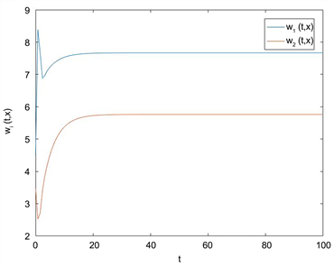
Figure 1. State track of the system (8)

图1. 系统(8)的状态轨迹

5. 小结

本文利用压缩映射理论研究了一类具有时变时滞的分数阶模糊细胞神经网络稳定性问题。模糊细胞神经网络在图像识别领域有着其独特的存在地位，我们在基本的时滞模糊细胞神经网络上，引入分数阶导数的定义，利用不同于构造Lyapunov函数的方法得到其稳定性判据，使所得结果比以往更为简洁和广泛。该模型的分析可以应用于工程、生物学和医学的不同类别分数阶神经网络模型的定性理论。

基金项目

这项研究得到云南省教育厅科学研究基金(2023Y0660)、运筹与优化硕士生导师团队，2021年云南省研究生导师团队建设项目、面向RCEP的跨境贸易区块链关键技术研究(202202AD080011)、云南省跨境贸易与金融区块链国际联合研发中心(202203AP140010)资助。

NOTES

^*通讯作者。

参考文献

[1]	Duan, L., Wei, H. and Huang, L. (2019). Finite-Time Synchronization of Delayed Fuzzy Cellular Neural Networks with Discontinuous Activations. Fuzzy Sets and Systems, 361, 56-70. https://doi.org/10.1016/j.fss.2018.04.017
[2]	Wang, F.C. and Liao, T.L. (2000). Global Stability for Cellular Neural Networks with Time Delay. IEEE Transactions on Neural Networks, 11, 1481-1484. https://doi.org/10.1109/72.883480
[3]	Chua, L.O. and Yang, L. (1988) Cellular Neural Networks: Theory. IEEE Transactions on Circuits and Systems, 35, 1257-1272. https://doi.org/10.1109/31.7600
[4]	Roska, T. and Chua, L.O. (1992) Cellular Neural Networks with Nonlinear and Delay-Type Template Elements and Nonuniform Grids. In-ternational Journal of Circuit Theory and Applications, 20, 469-481. https://doi.org/10.1002/cta.4490200504
[5]	Harrer, H. and Nossek, J.A. (1992) Discrete-Time Cellular Neural Networks. International Journal of Circuit Theory and Applications, 20, 453-467. https://doi.org/10.1002/cta.4490200503
[6]	Yang, T., Yang, L.B., Wu, C.W. and Chua, L.O. (1996) Fuzzy Cel-lular Neural Networks: Theory. 1996 Fourth IEEE International Workshop on Cellular Neural Networks and their Ap-plications Proceedings (CNNA-96), Seville, 24-26 June 1996, 181-186.
[7]	Huang, Z.D. (2016) Almost Periodic Solu-tions for Fuzzy Cellular Neural Networks with Multi-Proportional Delays. International Journal of Machine Learning and Cybernetics, 8, 1323-1331. https://doi.org/10.1007/s13042-016-0507-1
[8]	Wang, S.T. and Wang, M. (2006) A New Detection Algorithm Based on Fuzzy Cellular Neural Networks for White Blood Cell Detection. IEEE Trans-actions on Information Technology in Biomedicine, 10, 5-10. https://doi.org/10.1109/TITB.2005.855545
[9]	Ma, W.Y., Li, C.P. and Wu, Y.J. (2016) Impulsive Synchroniza-tion of Fractional Takagi-Sugeno Fuzzy Complex Networks. Chaos, 26, Article ID: 084311. https://doi.org/10.1063/1.4959535
[10]	Singh, A. and Rai, J.N. (2021) Stability Analysis of Fractional Order Fuzzy Cellular Neural Networks with Leakage Delay and Time Varying Delays. Chinese Journal of Physics, 73, 589-599. https://doi.org/10.1016/j.cjph.2021.07.029
[11]	Shen, H., Li, F., Yan, H., Karimi, H.R. and Lam, H.K. (2018) Finite-Time Event-Triggered H∞ Control for T-S Fuzzy Markov Jump Systems. IEEE Transactions on Fuzzy Systems, 26, 3122-3135. https://doi.org/10.1109/TFUZZ.2017.2788891
[12]	Shen, H., Li, F., Wu, Z., Park, J.H. and Sreeram, V. (2018) Fuzzy-Model-Based Non-Fragile Control for Nonlinear Singularly Perturbed Systems with Semi-Markov Jump Parame-ters. IEEE Transactions on Fuzzy Systems, 26, 3428-3439. https://doi.org/10.1109/TFUZZ.2018.2832614
[13]	Bas, E., Egrioglu, E. and Cansu, T. (2024) Robust Training of Median Dendritic Artificial Neural Networks for Time Series Forecasting. Expert Systems with Applications, 238, Article ID: 122080. https://doi.org/10.1016/j.eswa.2023.122080
[14]	Zhang, Y., Abdullah, S., Ullah, I. and Ghani, F. (2024) A New Approach to Neural Network via Double Hierarchy Linguistic Information: Application in Robot Selection. Engineering Applications of Artificial Intelligence, 129, Article ID: 107581. https://doi.org/10.1016/j.engappai.2023.107581
[15]	Guo, X.H., Zhou, L., Guo, Q. and Rouyendegh, B.D. (2021) An Optimal Size Selection of Hybrid Renewable Energy System Based on Fractional-Order Neural Network Algorithm: A Case Study. Energy Reports, 7, 7261-7272. https://doi.org/10.1016/j.egyr.2021.10.090
[16]	张硕. 基于李雅普诺夫方法的分数阶神经网络动力学分析及控制[D]: [博士学位论文]. 北京: 北京交通大学, 2017.
[17]	Stamova, I., Stamov, T. and Stamov, G. (2022) Lipschitz Stability Analysis of Fractional-Order Impulsive Delayed Reaction-Diffusion Neural Network Models. Chaos, Solitons and Fractals, 162, Article ID: 112474. https://doi.org/10.1016/j.chaos.2022.112474
[18]	罗欢, 郝冰, 陈付彬. Caputo分数阶时滞细胞神经网络的稳定性分析[J]. 数学的实践与认识, 2022, 52(7): 248-255.
[19]	Stamov, T. and Stamova, I. (2021) Design of Impulsive Controllers and Impulsive Control Strategy for the Mittag-Leffler Stability Behavior of Fractional Gene Regulatory Networks. Neurocomputing, 424, 54-62. https://doi.org/10.1016/j.neucom.2020.10.112
[20]	Shafiya, M. and Nagamani, G. (2022) New Finite-Time Pas-sivity Criteria for Delayed Fractionalorder Neural Networks Based on Lyapunov Function Approach. Chaos, Solitons & Fractals, 158, Article ID: 112005. https://doi.org/10.1016/j.chaos.2022.112005
[21]	Stamova, I. and Stamov, G. (2017) Mittag-Leffler Synchroniza-tion of Fractional Neural Networks with Time-Varying Delays and Reaction-Diffusion Terms Using Impulsive and Linear Controllers. Neural Networks, 96, 22-32. https://doi.org/10.1016/j.neunet.2017.08.009
[22]	牟天伟, 饶若峰. 不动点原理在时滞BAM神经网络稳定性分析中的一个应用[J]. 西南大学学报(自然科学版), 2017, 39(6): 5-9.
[23]	Rao, R.F., Zhong, S.M. and Pu, Z.L. (2019) Fixed Point and P-Stability of T-S Fuzzy Impulsive Reaction-Diffusion Dynamic Neural Networks with Dis-tributed Delay via Laplacian Semigroup. Neurocomputing, 335, 170-184. https://doi.org/10.1016/j.neucom.2019.01.051
[24]	Pu, Z.L. and Rao, R.F. (2018) Exponential Stability Criterion of High-Order BAM Neural Networks with Delays and Impulse via Fixed Point Approach. Neurocomputing, 292, 63-71. https://doi.org/10.1016/j.neucom.2018.02.081
[25]	Kilbas, A., Srivastava, H. and Trujillo, J. (2006) Theory and Applications of Fractional Differential Equations. Elsevier, Amsterdam.
[26]	唐致娣, 赵廷刚. 两种近似计算Caputo导数的有限差分方法[J]. 温州大学学报(自然科学版), 2013, 34(2): 1-6.

为你推荐

友情链接