基于非均匀网格的预测校正法求解非线性分数阶常微分方程初值问题
A Predictor-Corrector Method for Nonlinear Fractional Differential Equation Initial Value Problems on Graded Grids
DOI: 10.12677/AAM.2023.1212483, PDF, HTML, XML, 下载: 127  浏览: 220 
作者: 李一丹:贵州师范大学数学科学学院,贵州 贵阳
关键词: 二次插值分数阶微分方程非均匀网格预测校正法Quadratic Interpolation Fractional Differential Equation Graded Grid Predictor-Corrector Method
摘要: 非线性分数阶微分方程初值问题的典型解在初始时刻具有弱奇异性,为了更好地逼近它的典型解,本文将Nguyen和Jang在均匀网格上的三阶预测校正方法推广到非均匀网格上。与文献中现有的预测校正方法相比,这种新方法在降低计算成本的同时,显著提高了数值精度。另外,通过数值算例得到的结果显示,当选择合适的网格参数时,误差的收敛阶大于3。
Abstract: In order to better approximate the classical solution of nonlinear fractional differential equation in-itial value problems, which has weak singularity at the initial time, the third order predictor- cor-rector method of Nguyen and Jang on uniform grids is extended to non-uniform grids. Compared with the existing predictor-corrector methods in the literature, this new method reduces the com-putation cost and significantly improves the numerical accuracy. In addition, numerical examples show that the convergence order of errors is greater than the third order when appropriate mesh parameters are selected.
文章引用:李一丹. 基于非均匀网格的预测校正法求解非线性分数阶常微分方程初值问题[J]. 应用数学进展, 2023, 12(12): 4907-4913. https://doi.org/10.12677/AAM.2023.1212483

1. 引言

近年来,由于分数阶微分方程在物理学和工程学中的各种应用,引起了研究人员的广泛关注。例如,学者普遍感兴趣的分数阶模型包括分数阶反常扩散模型 [1] - [6] 、分数阶水波模型 [7] 、分数阶Cable模型 [8] 、分数阶Allen-Cahn方程 [9] 、分数阶Bloch-Torrey方程 [10] [11] 、分数阶扩散波动方程 [12] [13] [14] [15] [16] 等。由于分数阶导数本身具有的历史性和非局部特性,所以寻找其精度较高的数值算法变得尤为重要。

Adams方法具有稳定性好、计算量合理、易于实现等优点,是常微分方程数值解的一种常用的离散方法。为了将这些方法推广到分数阶微分方程,已经做了大量的工作。Diethelm和他的合著者 [17] [18] [19] [20] 研究了一种使用Adam公式的预测–校正方法,并对均匀网格进行了详细的误差分析。随后,Liu,Roberts和Yan将这种预测校正方法推广到非均匀网格 [21] 。

对于非线性分数阶常微分方程初值问题,Nguyen和Jang [22] 提出了均匀网格上的预测–校正法,该方法以较低的计算成本获得了较高的精度。但是该类问题的主要困难之处是典型解在初始时具有弱奇异性,为了解决数值解中的这一困难,Zhou和Li [23] 将 [22] 的Adams型预测–校正方法推广到非均匀网格上,在近似方法中只采用了线性插值。我们在这些基础上,将采用二次插值的Adams型预测校正方法推广到了非均匀网格上,通过数值算例得到的结果显示,当选择合适的网格参数时,误差的收敛阶大于3。

2. 主要内容

在本篇文章中,我们要研究的分数阶微分方程如下

{ D 0 α y ( t ) = f ( t , y ( t ) ) , 0 < t T , y ( 0 ) = y 0 . (1)

其中 α ( 0 , 1 ) D 0 α y ( t ) α 阶Caputo导数,即

D 0 α y ( t ) = 1 Γ ( 1 α ) 0 t ( t τ ) α y ( τ ) d τ (2)

众所周知,一个连续函数 y ( t ) 是方程(1)的解当且仅当它是Volterra积分方程 [24] 的解,所以我们有

y ( t ) = y 0 + 1 Γ ( α ) 0 t ( t τ ) α 1 f ( τ , y ( τ ) ) d τ (3)

这里的Volterra积分方程的理论分析和数值方法可以参考 [24] 和 [25] 等文献。

在本研究中,我们采取的是以下网格:N是任意正整数,将 [ 0 , T ] 区间划分为N个子区间,网格点

t n : = T ( n N ) r 0 n N ,r是待选择的网格分级参数。

在网格点 t = t n + 1 处,可改写(3)为

y ( t n + 1 ) = y 0 + 1 Γ ( α ) j = 0 n 1 t j t j + 1 ( t τ ) α 1 f ( τ , y ( τ ) ) d τ + 1 Γ ( α ) t n t n + 1 ( t τ ) α 1 f ( τ , y ( τ ) ) d τ y 0 + F h ( t n + 1 ) + F l ( t n + 1 ) (4)

这里的 F h ( t n + 1 ) F l ( t n + 1 ) 分别表示Volterra积分算子的历史部分和局部部分。

本篇文章中将在分级网格上来讨论二次插值的预测校正方法,通过与均匀网格的对比体现了本方案的优越性,具体操作在第3节中会作详细介绍。

3. 二次插值的预测校正方法

为方便起见,定义 y j = y ( t j ) 为解在 t j 处的精确解, j = 0 , , N 。定义 y ˜ j + 1 P y ˜ j + 1 y j + 1 分别是 y j + 1 的预测校正值和近似校正值。类似地可定义 f j = f ( t j , y j ) f ˜ j = f ˜ ( t j , y j ) 以及 f ˜ P j = f ( t j , y ˜ P j ) 。Volterra积分算子的历史部分 F h ( t n + 1 ) 和局部部分 F l ( t n + 1 ) 分别用 F ˜ h ( t n + 1 ) F ˜ l ( t n + 1 ) 来近似。

在每个区间 [ t j 1 , t j + 1 ] 上,这里 j 1 ,我们用二次拉格朗日插值来逼近 f ( t ) ,即:

f ( t ) f j 1 ( t t j ) ( t t j + 1 ) ( t j 1 t j ) ( t j 1 t j + 1 ) + f j ( t t j 1 ) ( t t j + 1 ) ( t j t j 1 ) ( t j t j + 1 ) + f j + 1 ( t t j 1 ) ( t t j ) ( t j + 1 t j 1 ) ( t j + 1 t j ) (5)

再来处理区间 [ t 0 , t 1 ] f ( t ) 在该区间上可用

f ( t ) f 0 ( t t 1 / 2 ) ( t t 1 ) ( t 0 t 1 / 2 ) ( t 0 t 1 ) + f 1 / 2 ( t t 0 ) ( t t 1 ) ( t 1 / 2 t 0 ) ( t 1 / 2 t 1 ) + f 1 ( t t 0 ) ( t t 1 / 2 ) ( t 1 t 0 ) ( t 1 t 1 / 2 ) (6)

来近似。将上述两式代入(4)式中,我们得到

y ˜ n + 1 = y 0 + F ˜ h ( t n + 1 ) + F ˜ l ( t n + 1 ) (7)

这里的记忆部分

F ˜ h ( t n + 1 ) = 1 Γ ( α ) [ A n + 1 0 , 0 f ˜ 0 + A n + 1 1 , 0 f ˜ 1 / 2 + A n + 1 2 , 0 f ˜ 1 ] + 1 Γ ( α ) j = 1 n 1 [ A n + 1 0 , j f ˜ j 1 + A n + 1 1 , j f ˜ j + A n + 1 2 , 0 f ˜ j + 1 ] (8)

以及局部部分

F ˜ l ( t n + 1 ) = 1 Γ ( α ) [ A n + 1 0 , n f ˜ n 1 + A n + 1 1 , n f ˜ n + A n + 1 2 , n f ˜ n + 1 P ] (9)

其中的预测近似值 y ˜ n + 1 P 用(10)式来近似,即在区间 [ t n , t n + 1 ] 上用 f ˜ n 2 f ˜ n 1 以及 f ˜ n 的二次插值来逼近 f ( t )

y ˜ n + 1 P = y 0 + F ˜ h ( t n + 1 ) + 1 Γ ( α ) [ b n + 1 0 , n f ˜ n 2 + b n + 1 1 , n f ˜ n 1 + b n + 1 2 , n f ˜ n ] (10)

下面是需要计算的系数部分,计算公式如下

A n + 1 0 , 0 = t 0 t 1 ( t n + 1 t ) α 1 ( t t 1 / 2 ) ( t t 1 ) ( t 0 t 1 / 2 ) ( t 0 t 1 ) d t A n + 1 1 , 0 = t 0 t 1 ( t n + 1 t ) α 1 ( t t 0 ) ( t t 1 ) ( t 1 / 2 t 0 ) ( t 1 / 2 t 1 ) d t

A n + 1 2 , 0 = t 0 t 1 ( t n + 1 t ) α 1 ( t t 0 ) ( t t 1 / 2 ) ( t 1 t 0 ) ( t 1 t 1 / 2 ) d t b n + 1 0 , n = t n t n + 1 ( t n + 1 t ) α 1 ( t t n 1 ) ( t t n ) ( t n 2 t n 1 ) ( t n 2 t n ) d t

b n + 1 1 , n = t n t n + 1 ( t n + 1 t ) α 1 ( t t n 2 ) ( t t n ) ( t n 1 t n 2 ) ( t n 1 t n ) d t b n + 1 0 , n = t n t n + 1 ( t n + 1 t ) α 1 ( t t n 1 ) ( t t n ) ( t n 2 t n 1 ) ( t n 2 t n ) d t

其余需计算的系数如下(其中 j = 1 , , n )

A n + 1 0 , j = t j t j + 1 ( t n + 1 t ) α 1 ( t t j ) ( t t j + 1 ) ( t j 1 t j ) ( t j 1 t j + 1 ) d t A n + 1 0 , j = t j t j + 1 ( t n + 1 t ) α 1 ( t t j 1 ) ( t t j + 1 ) ( t j t j 1 ) ( t j t j + 1 ) d t

A n + 1 2 , j = t j t j + 1 ( t n + 1 t ) α 1 ( t t j 1 ) ( t t j ) ( t j + 1 t j 1 ) ( t j + 1 t j ) d t

上述过程可归结为以下:

{ y ˜ n + 1 = y 0 + F ˜ h ( t n + 1 ) + F ˜ l ( t n + 1 ) y ˜ n + 1 P = y 0 + F ˜ h ( t n + 1 ) + 1 Γ ( α ) [ b n + 1 0 , n f ˜ n 2 + b n + 1 1 , n f ˜ n 1 + b n + 1 2 , n f ˜ n ] F ˜ l ( t n + 1 ) = 1 Γ ( α ) [ A n + 1 0 , n f ˜ n 1 + A n + 1 1 , n f ˜ n + A n + 1 2 , n f ˜ n + 1 P ] F ˜ h ( t n + 1 ) = 1 Γ ( α ) [ A n + 1 0 , 0 f ˜ 0 + A n + 1 1 , 0 f ˜ 1 / 2 + A n + 1 2 , 0 f ˜ 1 ] + 1 Γ ( α ) j = 1 n 1 [ A n + 1 0 , j f ˜ j 1 + A n + 1 1 , j f ˜ j + A n + 1 2 , 0 f ˜ j + 1 ] (11)

另外,在计算的循环过程启动之前,我们还须计算 y ˜ 1 y ˜ 2 这两个值,具体的计算过程如下:

1) L 0 ( f ˜ 0 ) y ˜ 1 / 4 P L 1 ( f ˜ 0 , f ˜ 1 / 4 P ) y ˜ 1 / 4

2) L 1 ( f ˜ 0 , f ˜ 1 / 4 ) F ˜ h ( t 1 / 2 ) ; L 0 ( f ˜ 1 / 4 ) y ˜ 1 / 2 P 1 L 1 ( f ˜ 1 / 4 , f ˜ 1 / 2 P 1 ) y ˜ 1 / 2 P 2 L 2 ( f ˜ 0 , f ˜ 1 / 4 , f ˜ 1 / 2 P 2 ) y ˜ 1 / 2

3) L 1 ( f ˜ 0 , f ˜ 1 / 2 ) F ˜ h ( t 1 ) ; L 0 ( f ˜ 1 / 2 ) y ˜ 1 P 1 L 1 ( f ˜ 1 / 2 , f ˜ 1 P 1 ) y ˜ 1 P 2 L 2 ( f ˜ 0 , f ˜ 1 / 2 , f ˜ 1 P 2 ) y ˜ 1

4) L 2 ( f ˜ 0 , f ˜ 1 / 2 , f ˜ 1 ) F ˜ h ( t 2 ) ; L 0 ( f ˜ 1 ) y ˜ 2 P 1 L 1 ( f ˜ 1 , f ˜ 2 P 1 ) y ˜ 2 P 2 L 2 ( f ˜ 0 , f ˜ 1 , f ˜ 2 P 2 ) y ˜ 2

其中 L 0 ( f a ) 为f在 t = a 处的常数插值即 L 0 ( f a ) = f ( a ) L 1 ( f a , f b ) 为f在网格 ( a , b ) 处的线性插值, L 2 ( f a , f b , f c ) 为f在网格 ( a , b , c ) 处的二次插值,此启动方案参照文献 [22] 。

4. 数值实验

在本小节中,我们给出了一个数值例子来说明均匀网格上与非均匀网格上的二次插值预测校正方法的收敛阶数。

例1考虑如下分数阶微分方程

{ D 0 α y ( t ) = Γ ( 4 + α ) 6 t 3 + t 3 + α y ( t ) , 0 < t T y ( 0 ) = 0

该问题的精确解为: y ( t ) = t 3 + α

图1是当 α = 0.4 , r = 1 + α 2 α 时,例1的精确解与数值解的图像。由图可以看出,我们采取的方法所算

出的值几乎与精确解的函数值吻合,证明了该方法的有效性。

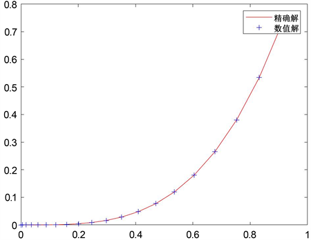
Figure 1. Image of the exact and numerical solution of example 1 when N = 20

图1. 当N = 20时例1的精确解与数值解的图像

表1表示用均匀网格上与分级网格上的二次插值预测校正方法来计算例1的最大节点误差及收敛阶

(其中 α = 0.4 )。另外 e r r N : = max 0 j N | y ( t j ) y j | p N : = log 2 ( e r r N / e r r 2 N )

Table 1. The maximum node error and convergence order of example 1

表1. 例1的最大节点误差及收敛阶

例2考虑如下非线性分数阶微分方程

{ D 0 α y ( t ) = Γ ( 4 + α ) 6 t 3 + t 6 + 2 α y 2 ( t ) , 0 < t T y ( 0 ) = 0

该问题的精确解为: y ( t ) = t 3 + α

同样地,我们画出例2的精确解和数值解图像如图2。可以看出图像基本吻合,这表明我们的方法可以去计算这样的非线性分数阶微分方程初值问题。

表1表2,当 r = 1 时即取均匀网格时, p N 随着N的增大却在减小,对比 r = 1 + α 2 α 时, p N 随着N

的增大而增大,并且数值略大于均匀网格时的情形。因此,非均匀网格的收敛阶优于均匀网格的收敛阶,这个数值结果证明了方法的优越性。

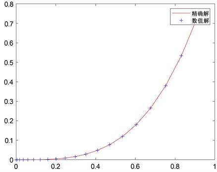
Figure 2. Image of the exact and numerical solution of example 2 when N = 20

图2. 当N = 20时例2的精确解与数值解的图像

Table 2. The maximum node error and convergence order of example 2

表2. 例2的最大节点误差及收敛阶

5. 结论

分数阶常微分方程在数学模型中的应用受到越来越广泛的关注。不同的分数阶常微分方程模型已被应用到越来越多的领域中。并且发现它在研究一些具有记忆过程、遗传性质以及异质材料时比整数阶方程模型更有优势。本文研究的问题是非线性分数阶初值问题的数值解,我们将Nguyen和Jang的三阶预测校正方法推广到非均匀网格上,主要是在非均匀网格上进行二次插值,然后用预测校正法进行求解,数值实验表明误差阶超过三阶,我们接下来的工作将对本文所提出的数值方法进行误差分析并用于求解分数阶偏微分方程。

参考文献

[1] Liu, Y., Du, Y., Li, H., He, S. and Gao, W. (2015) Finite Difference/Finite Element Method for a Nonlinear Time- Frac-tional Fourth-Order Reaction-Diffusion Problem. Computers & Mathematics with Applications, 70, 573-591.
https://doi.org/10.1016/j.camwa.2015.05.015
[2] Shi, D. and Yang, H. (2018) Superconvergence Analysis of a New Low Order Nonconforming MFEM for Time-Fractional Diffusion Equation. Applied Numerical Mathematics, 131, 109-122.
https://doi.org/10.1016/j.apnum.2018.05.002
[3] Deng, W., Li, C. and Guo, Q. (2007) Analysis of Fractional Differential Equations with Multi-Orders. Fractals, 15, 173-182.
https://doi.org/10.1142/S0218348X07003472
[4] Liu, Y. and Xu, C. (2007) Finite Difference/Spectral Approxi-mations for the Time-Fractional Diffusion Equation. Journal of Computational Physics, 225, 1533-1552.
https://doi.org/10.1016/j.jcp.2007.02.001
[5] Yue, X., Shu, S., Xu, X., Bu, W. and Pan, K. (2019) Paral-lel-in-Time Multigrid for Space-Time Finite Element Approximations of Two-Dimensional Space-Fractional Diffusion Equation. Computers & Mathematics with Applications, 78, 3471-3484.
https://doi.org/10.1016/j.camwa.2019.05.017
[6] Zheng, M., Liu, F., Liu, Q., Burrage, K. and Simpson, M.J. (2017) Numerical Solution of the Time Fractional Reaction- Diffusion Equation with a Moving Boundary. Journal of Computational Physics, 338, 493-510.
https://doi.org/10.1016/j.jcp.2017.03.006
[7] Liu, Y., Yu, Z., Li, H., Liu, F. and Wang, J. (2018) Time Two-Mesh Algorithm Comblined with Finite Element Method for Time Fractional Water Wave Model. International Journal of Heat and Mass Transfer, 120, 1132-1145.
https://doi.org/10.1016/j.ijheatmasstransfer.2017.12.118
[8] Liu, Y., Du, Y., Li, H. and Wang, J. (2016) A Two-Grid Finite Element Approximation for a Nonlinear Time-Fractional Cabel Equation. Nonlinear Dynamics, 85, 2535-2548.
https://doi.org/10.1007/s11071-016-2843-9
[9] Yin, B., Liu, Y., Li, H. and He, S. (2019) Fast Algo-rithm Based on TT-M FE System for Space Fractional Allen-Cahn Equations with Smooth and Non-Smooth Solution. Journal of Computational Physics, 379, 351-372.
https://doi.org/10.1016/j.jcp.2018.12.004
[10] Bu, W., Tang, Y., Wu, Y. and Yang, J. (2015) Finite Differ-ence/Finite Element Method for Two Dimensional Space and Time Fractional Bloch-Torrey Equations. Journal of Com-putational Physics, 293, 264-279.
https://doi.org/10.1016/j.jcp.2014.06.031
[11] Yang, Z., Liu, F., Nie, Y. and Turner, I. (2020) An Unstructured Mesh Finite Difference /Finite Element Method for the Three-Dimensional Time-Space Fractional Bloch-Torrey Equa-tions on Irregular Domain. Journal of Computational Physics, 408, Article ID: 109284.
https://doi.org/10.1016/j.jcp.2020.109284
[12] Ding, H. and Li, C. (2013) Numerical Algorithms for the Fractional Diffusion-Wave Equation with Reaction Term. Abstract and Applied Analysis, 2013, Article ID: 493406.
https://doi.org/10.1155/2013/493406
[13] Luo, Z. and Wang, H. (2020) A Highly Efficient Reduced-Order Extrap-olated Finite Difference Algorithm for Time-Space Tempered Fractional Diffusion-Wave Equation. Applied Mathematics Letters, 102, Article ID: 106090.
https://doi.org/10.1016/j.aml.2019.106090
[14] Sun, Z. and Wu, X. (2006) A Fully Discrete Difference Scheme for a Diffusion-Wave System. Applied Numerical Mathematics, 56, 193-209.
https://doi.org/10.1016/j.apnum.2005.03.003
[15] Liu, L., Xu, D. and Luo, M. (2013) Alternating Direction Implic-it Galerkin Finite Element Method for Two-Dimensional Fractional Diffusion-Wave Equation. Journal of Computational Physics, 255, 471-485.
https://doi.org/10.1016/j.jcp.2013.08.031
[16] Jin, B.T., Lazarov, R. and Zhou, Z. (2016) Two Fully Discrete Schemes for Fractional Diffusion-Wave Equations with Nonsmooth Date. SIAM Journal on Scientific Computing, 38, A146-A170.
https://doi.org/10.1137/140979563
[17] Stynes, M., O’Riordan, E. and Gracia, J.L. (2017) Error Analysis of a Finite Difference Method on Graded Meshes for a Time-Fractional Diffusion Equation. SIAM Journal on Numerical Analysis, 55, 1057-1079.
https://doi.org/10.1137/16M1082329
[18] Diethelm, K. and Freed, A.D. (1999) The Fracpece Subroutine for the Numerical Solution of Differential Equations of Fractional Order. Forschung und wissenschaftliches Rechnen, Göttingen, 57-71.
[19] Diethelm, K., Ford, N.J. and Freed, A.D. (2002) A Predictor-Corrector Approach for the Numerical Solu-tion of Fractional Differential Equations. Nonlinear Dynamics, 29, 3-22.
https://doi.org/10.1023/A:1016592219341
[20] Diethelm, K. and Ford, N.J. (2022) Analysis of Fractional Differ-ential Equations. Journal of Mathematical Analysis and Applications, 265, 229-248.
https://doi.org/10.1006/jmaa.2000.7194
[21] Diethelm, K., Ford, N.J. and Freed, A.D. (2004) Detailed Error Anal-ysis for a Fractional Adams Method. Numerical Algorithms, 36, 31-52.
https://doi.org/10.1023/B:NUMA.0000027736.85078.be
[22] Liu, Y.Z., Roberts, J. and Yan, Y.B. (2018) A Note on Finite Difference Methods for Nonlinear Fractional Differential Equations with Non-Uniform Meshes. International Journal of Computer Mathematics, 95, 1151-1169.
https://doi.org/10.1080/00207160.2017.1381691
[23] Zhou, Y., Li, C. and Stynes, M. (2022) A Fast Sec-ond-Order Predictor-Corrector Method for a Nonlinear Time-Fractional Benjamin-Bona-Mahony-Burgers Equation. Numerical Algorithms.
https://doi.org/10.1007/s11075-023-01586-x
[24] Capobianco, G., Conte, D., Del Prete, I. and Russo, E. (2007) Fast RungeKutta Methods for Nonlinear Convolution Systems of Voterra Integral Equations. BIT Numerical Mathematics, 47, 259-275.
https://doi.org/10.1007/s10543-007-0120-5
[25] Conte, D. and Prete, I.D. (2006) Fast Collocation Methods for Volterra Integral Equations of Convolution Type. Journal of Computational and Applied Mathematics, 196, 652-663.
https://doi.org/10.1016/j.cam.2005.10.018