二阶BDF2压力修正投影方法求解扩散Peterlin粘弹性流体

Second Order BDF2 Pressure Correction Projection Method Solving Diffusive Peterlin Viscoelastic Fluid

摘要: 不可压扩散粘弹性流体是用来描述高分子聚合物的一类复杂流体。本文用二阶BDF2时间离散的压力修正投影方法求解扩散peterlin粘弹性流体。BDF2是三步格式，具有2阶收敛精度。压力修正投影方法用来避开流体速度和压力的耦合的不可压约束条件∇-u=0。当时间步长Δt小于给定常数时，我们证明了该方法无条件稳定。最后数值算例验证了格式的稳定性。

Abstract: The incompressible peterlin diffusive viscoelastic fluid is one type of complex fluid which used to describe high-molecular polymer. Second order time discrete BDF2 pressure correction projection method is to solve the diffusive peterlin viscoelastic model in this paper. BDF2 is three step steps scheme, and it has second order accuracy. Pressure correction projection method is used to avoid the incompressible restriction ∇-u=0 between the fulid velocity u and the pressure p. We prove that the method is unconditional stability if time step Δt less than a constant. Finally, we present some numerical experiment to verify the stability.

1. 引言

粘弹性流体 [1] 存在于日常生活的方方面面，比如，食物中的番茄酱，蛋黄酱等，熔化的塑料，生物流体等。在工业上，向水中加入水溶性高分子聚合物可以得到粘弹性流体。粘弹性流体不仅具有粘性属性，又具有弹性行为，是一种介于粘弹性流体与弹性固体之间的特殊流体。粘弹性流体属于非牛顿流体，有一些特殊的物理现象，比如weissenberg爬杆效应，剪切稀变效应等。

不可压扩散peterlin粘弹性流体模型 [2] [3] [4] [5] [6] 是由动量守恒的NS方程，质量守恒的不可压缩条件 $\nabla \cdot u=0$ 和利用peterlin 逼近描述构象张量d的本构方程耦合而成的，多变量、强非线性的方程组，如下

所示. 给定有界凸多边形区域 $\Omega \subset R^2$，有限时间T，求解速度u： $\Omega \times \left[0,T\right]\to R^2$，压力p： $\Omega \times \left[0,T\right]\to R$，对称构象张量d： $\Omega \times \left[0,T\right]\to R_{sym}^{2\times 2}$。

$\begin{array}{l}{\partial }_{t}u-\nu \Delta u+\left(u\cdot \nabla \right)u+\nabla p=\nabla \cdot \left[\left(trd\right)d\right]+f,\\ \nabla \cdot u=0,\\ {\partial }_{t}d-\epsilon \Delta d+\left(u\cdot \nabla \right)d=\left(\nabla u\right)d+d{\left(\nabla u\right)}^{\text{T}}+\left(trd\right)I-{\left(trd\right)}^{2}d+F,\end{array}$ (1)

其中 $trd$ 表示张量d的迹，I是单位矩阵。物理参数 $\nu >0$ 和 $\epsilon >0$ 分别表示流体粘性系数和弹性张量系

数。为了简单起见，速度u和构象张量d赋于Dirichlet齐次边界条件，即 ${u|}_{\partial \Omega }=0$， ${d|}_{\partial \Omega }=0$，并给定相

应的初始条件 $u\left(0,x\right)=u_0\left(x\right)$， $d\left(0,x\right)=d_0\left(x\right)$。

文献 [2] [3] 讨论了该流体模型解的存在唯一性以及正则性。关于该流体模型的数值研究，可看文献 [4] [5] [6] ，文献 [5] 讨论了问题(1)时间离散一阶欧拉线性化压力校正投影格式，并进行了稳定化和先验误差分析。本文将继续讨论问题(1)的时间离散二阶BDF2压力校正投影格式。BDF2是线性多步法中的3步方法 [7] ，具有2阶收敛精度。压力修正投影格式，首先是由Chorin在1960年提出的 [8] ，主要是为了避开不可压缩流体的不可压条件。关于该方法针对不可压缩流体的综述文章见文献 [9] 。

本文结构如下。第二节给出该流体模型相应的预备知识和二阶压力校正投影格式。第三节对二阶BDF2压力校正投影格式进行了稳定性分析。第四节给出数值算例验证格式的稳定性。最后给出了小结。

2. 预备知识和数值格式

设 $L^r\left(\Omega \right)$ 表示区域 $\Omega$ 上的勒贝格空间，其范数为 ${\Vert \cdot \Vert }_{L^r\left(\Omega \right)}$。符号 $\Vert \cdot \Vert$ 和 ${\Vert \cdot \Vert }_{\infty }$ 分别表示 $L^2\left(\Omega \right)$ 和 $L^{\infty }\left(\Omega \right)$ 空间的范数。 $H^k\left(\Omega \right)$ 表示索伯列夫空间 $W^{k,2}\left(\Omega \right)$，其范数为 ${\Vert \cdot \Vert }_k$。我们为了描述问题(1)的压力校正投影方

法，首先定义下列函数空间：

$H_0^1\left(\Omega \right)=\left\{\omega |\omega \in H^1\left(\Omega \right),{\omega |}_{\partial \Omega }=0\right\},L_0^2\left(\Omega \right)=\left\{q|q\in L^2\left(\Omega \right),{\displaystyle {\int }_{\Omega }q\text{d}\Omega }=0\right\}.$

为了给出问题(1)的时间离散BDF2压力修正投影方法，首先对时间区间[0, T]进行等距剖分。设 $0=t_0<t_1<\cdots <t_N=T$ 是区间[0, T]的等距剖分，时间步长为 $\Delta t$。记 $t_n=n\Delta t$ 和 ${\omega }^n=\omega \left(\cdot ,t_n\right)$。

格式2.1：(时间离散的BDF2压力校正投影)

第一步：通过下面的方程组求解 $\left({\tilde{u}}^{n+1},d^{n+1}\right)\in H_0^1{\left(\Omega \right)}^2\times H_0^1{\left(\Omega \right)}^{2\times 2}$

$\frac{3{\tilde{u}}^{n+1}-4u^n+u^{n-1}}{2\Delta t}-\nu \Delta {\tilde{u}}^{n+1}+\left({\tilde{u}}^{n+1}\cdot \nabla \right){\tilde{u}}^{n+1}+\nabla p^n=\nabla \cdot \left[\left(tr{d}^{n+1}\right)d^{n+1}\right]+f^{n+1},$ (2.1)

$\begin{array}{l}\frac{3d^{n+1}-4d^n+d^{n-1}}{2\Delta t}-\epsilon \Delta d^{n+1}+\left({\tilde{u}}^{n+1}\cdot \nabla \right)d^{n+1}\\ =\nabla {\tilde{u}}^{n+1}{d}^{n+1}+d^{n+1}{\left(\nabla {\tilde{u}}^{n+1}\right)}^{\text{T}}+\left(tr{d}^{n+1}\right)I-{\left(tr{d}^{n+1}\right)}^2{d}^{n+1}+F^{n+1}.\end{array}$ (2.2)

第二步：通过下面的方程组求解 $\left(u^{n+1},p^{n+1}\right)\in H_0^1{\left(\Omega \right)}^2\times L_0^2(\Omega )$

$\{\begin{array}{l}\frac{3u^{n+1}-3{\tilde{u}}^{n+1}}{2\Delta t}+\nabla \left(p^{n+1}-p^n\right)=0,\\ \nabla \cdot u^{n+1}=0.\end{array}$ (2.3)

注1. 由于BDF2是三步格式，需要知道前两步的函数值 $\left(u^0,d^0\right),\left(u^1,p^1,d^1\right)$。 我们可以用其它格式，例如Backward欧拉格式，得到 $\left(u^1,p^1,d^1\right)$。

注2. 由于格式2.1是非线性全隐格式，因此在后面的算例计算时，需要进行线性化迭代，这里我们采用Newton 迭代。

注3. 为了使压力与速度解耦计算，本文用了BDF2压力校正投影方法。第一步是关于中间速度 ${\tilde{u}}^{n+1}$ 和构象张量d的非线性椭圆型问题。第二步是关于速度和压力的线性方程组。

注4. 如果对第二步的第一个方程求散度 $\nabla \cdot$，可以得到 $-\frac{3\nabla \cdot {\tilde{u}}^{n+1}}{2\Delta t}+\Delta \left(p^{n+1}-p^n\right)=0$，即 $-\Delta p^{n+1}=-\frac{3}{2\Delta t}\nabla \cdot {\tilde{u}}^{n+1}-\Delta p^n$。这是一个关于压力的Possion方程。在求得压力 $p^{n+1}$ 后，可以通过下式得到

最终速度 $u^{n+1}$

$u^{n+1}={\tilde{u}}^{n+1}-\frac{2}{3}\Delta t\nabla \left(p^{n+1}-p^n\right).$

于是时间离散的BDF2压力校正投影格式2.1，可以写成三步形式。

格式2.2：(时间离散的BDF2压力校正投影三步方法)

第一步：与格式2.1的第一步相同

第二步：通过下面的方程求解压力 $p^{n+1}\in L_0^2\left(\Omega \right)\cap H^1(\Omega )$

$-\Delta p^{n+1}=-\frac{3}{2\Delta t}\nabla \cdot {\tilde{u}}^{n+1}-\Delta p^n.$

第三步：通过下面的方程求解速度 $u^{n+1}\in H_0^1{\left(\Omega \right)}^2$

$u^{n+1}={\tilde{u}}^{n+1}-\frac{2}{3}\Delta t\nabla \left(p^{n+1}-p^n\right).$

3. 二阶BDF2压力校正投影格式2.1的稳定性分析

定理3.1. 设 $\left(u^{n+1},{\tilde{u}}^{n+1},p^{n+1}\right)$ 是数值格式2.1的解。格式2.1几乎无条件稳定，即当时间步长 $\Delta t\le \frac{1}{16}$ 时，

有下面的稳定性结论

$\begin{array}{l}{\Vert u^N\Vert }^2+{\Vert 2u^N-u^{N-1}\Vert }^2+\frac{1}{2}{\Vert d^N\Vert }^2+\frac{1}{2}{\Vert d^N-d^{N-1}\Vert }^2+\frac{4}{3}{\left(\Delta t\right)}^2{\Vert \nabla p^N\Vert }^2\\ +2\Delta t\nu {\displaystyle \underset{n=1}{\overset{N-1}{\sum }}{\Vert \nabla {\tilde{u}}^{n+1}\Vert }^2}+2\Delta t{\displaystyle \underset{n=1}{\overset{N-1}{\sum }}{\Vert \left(tr{d}^{n+1}\right)d^{r+1}\Vert }^2}\\ \le \exp \left(2T\right)\{{\Vert u^1\Vert }^2+{\Vert 2u^1-u^0\Vert }^2+\frac{1}{2}{\Vert d^1-d^0\Vert }^2+\frac{4}{3}{\left(\Delta t\right)}^2{\Vert \nabla p^1\Vert }^2\\ +\Delta t{\displaystyle \underset{n=1}{\overset{N-1}{\sum }}\left[\frac{2}{\nu }{\Vert f^{n+1}\Vert }_{-1}^2+\frac{1}{\epsilon }{\Vert F^{n+1}\Vert }_{-1}^2\right]}\}.\end{array}$ (3.1)

证明. 方程(2.1)两端乘以 $4\Delta t{\tilde{u}}^{n+1}$ 并在区域 $\Omega$ 上积分，利用Green公式和三线性项 $\left({\tilde{u}}^{n+1}\cdot \nabla {\tilde{u}}^{n+1},{\tilde{u}}^{n+1}\right)=0$，我们得到

$\begin{array}{l}\left(3{\tilde{u}}^{n+1}-4u^n+u^{n-1},2{\tilde{u}}^{n+1}\right)+4\Delta t\nu {\Vert \nabla {\tilde{u}}^{n+1}\Vert }^2+4\Delta t\left(\nabla p^n,{\tilde{u}}^{n+1}\right)\\ =-4\Delta t\left(\left(tr{d}^{n+1}\right)d^{n+1},\nabla {\tilde{u}}^{n+1}\right)+4\Delta t\left(f^{n+1},{\tilde{u}}^{n+1}\right).\end{array}$ (3.2)

同理，方程(2.2)两端乘以 $2\Delta t{d}^{n+1}$ 并在区域 $\Omega$ 上积分， 利用Green公式和三线性项 $\left({\tilde{u}}^{n+1}\cdot \nabla d^{n+1},d^{n+1}\right)=0$，我们得到

$\begin{array}{l}\left(3d^{n+1}-4d^n+d^{n-1},d^{n+1}\right)+2\Delta t\epsilon {\Vert \nabla d^{n+1}\Vert }^2\\ =2\Delta t\left(\nabla {\tilde{u}}^{n+1}{d}^{n+1}+d^{n+1}{\left(\nabla {\tilde{u}}^{n+1}\right)}^{{\rm T}},d^{n+1}\right)+2\Delta t{\Vert tr{d}^{n+1}\Vert }^2\\ -2\Delta t{\Vert \left(tr{d}^{n+1}\right)d^{n+1}\Vert }^2+2\Delta t\left(F^{n+1},d^{n+1}\right)\text{.}\end{array}$ (3.3)

方程(3.2)和(3.3)相加并且利用关系式 $2\left(\left(trd\right)d,\nabla u\right)=\left(\left(\nabla u\right)d+d{\left(\nabla u\right)}^{{\rm T}},d\right)$ 可得

$\begin{array}{l}\left(3{\tilde{u}}^{n+1}-4u^n+u^{n-1},2{\tilde{u}}^{n+1}\right)+\frac{1}{2}\left(3d^{n+1}-4d^n+d^{n-1},2d^{n+1}\right)+4\Delta t\nu {\Vert \nabla {\tilde{u}}^{n+1}\Vert }^2\\ +2\Delta t\epsilon {\Vert \nabla d^{n+1}\Vert }^2+4\Delta t\left(\nabla p^n,{\tilde{u}}^{n+1}\right)+2\Delta t{\Vert \left(tr{d}^{n+1}\right)d^{n+1}\Vert }^2\\ =2\Delta t{\Vert tr{d}^{n+1}\Vert }^2+4\Delta t\left(f^{n+1},{\tilde{u}}^{n+1}\right)+2\Delta t\left(F^{n+1},d^{n+1}\right).\end{array}$ (3.4)

我们首先对式子(3.4)的等号右端项进行估计。利用关系式 $2ab\le a^2+b^2$ 可得

$2\Delta t{\Vert tr{d}^{n+1}\Vert }^2\le 4\Delta t{\Vert d^{n+1}\Vert }^2\text{.}$ (3.5)

利用hölder和young’s不等式，我们得到

$4\Delta t\left(f^{n+1},{\tilde{u}}^{n+1}\right)\le 2\Delta t\nu {\Vert \nabla {\tilde{u}}^{n+1}\Vert }^2+\frac{2\Delta t}{\nu }{\Vert f^{n+1}\Vert }_{-1}^2,$ (3.6)

$2\Delta t\left(F^{n+1},d^{n+1}\right)\le \Delta t\epsilon {\Vert \nabla d^{n+1}\Vert }^2+\frac{\Delta t}{\epsilon }{\Vert F^{n+1}\Vert }_{-1}^2\text{.}$ (3.7)

将不等式估计(3.5)，(3.6)和(3.7)代入(3.4)可得：

$\begin{array}{l}\left(3{\tilde{u}}^{n+1}-4u^n+u^{n-1},2{\tilde{u}}^{n+1}\right)+\frac{1}{2}\left(3d^{n+1}-4d^n+d^{n-1},2d^{n+1}\right)+2\Delta t\nu {\Vert \nabla {\tilde{u}}^{n+1}\Vert }^2\\ +\epsilon \Delta t{\Vert \nabla d^{n+1}\Vert }^2+4\Delta t\left(\nabla p^n,{\tilde{u}}^{n+1}\right)+2\Delta t{\Vert \left(tr{d}^{n+1}\right)d^{n+1}\Vert }^2\\ \le 4\Delta t{\Vert d^{n+1}\Vert }^2+\frac{2\Delta t}{r}{\Vert f^{n+1}\Vert }_{-1}^2+\frac{\Delta t}{\epsilon }{\Vert F^{n+1}\Vert }_{-1}^2.\end{array}$ (3.8)

从格式2.1的第二步(2.3)，我们可以得到：

$3u^{n+1}+2\Delta t\nabla p^{n+1}=3{\tilde{u}}^{n+1}+2\Delta t\nabla p^n,$

对上式两边分别取内积，可得：

$4\Delta t\left({\tilde{u}}^{n+1},\nabla p^n\right)=3\left({\Vert u^{n+1}\Vert }^2-{\Vert {\tilde{u}}^{n+1}\Vert }^2\right)+\frac{4}{3}{\left(\Delta t\right)}^2\left({\Vert \nabla p^{n+1}\Vert }^2-{\Vert \nabla p^n\Vert }^2\right).$ (3.9)

应用关系式

$\begin{array}{l}\frac{1}{2}\left(3d^{n+1}-4d^n+d^{n-1},2d^{n+1}\right)\\ =\frac{1}{2}\left[{\Vert d^{n+1}\Vert }^2-{\Vert d^n\Vert }^2+{\Vert 2d^{n+1}-d^n\Vert }^2-{\Vert 2d^n-d^{n-1}\Vert }^2+{\Vert d^{n+1}-2d^n+d^{n-1}\Vert }^2\right];\end{array}$ (3.10)

和

$\begin{array}{l}\left(3{\tilde{u}}^{n+1}-4u^n+u^{n-1},2{\tilde{u}}^{n+1}\right)\\ =\left(3u^{n+1}-4u^n+u^{n-1},2u^{n+1}\right)-\left(3u^{n+1}-4u^n+u^{n-1},2\left(u^{n+1}-{\tilde{u}}^{n+1}\right)\right)\\ ={\Vert u^{n+1}\Vert }^2-{\Vert u^n\Vert }^2+{\Vert 2u^{n+1}-u^n\Vert }^2-{\Vert 2u^n-u^{n-1}\Vert }^2+{\Vert u^{n+1}-2u^n+u^{n-1}\Vert }^2\\ -3\left({\Vert u^{n+1}\Vert }^2-{\Vert {\tilde{u}}^{n+1}\Vert }^2-{\Vert u^{n+1}-{\tilde{u}}^{n+1}\Vert }^2\right).\end{array}$ (3.11)

我们将关系式(3.9)，(3.10)，(3.11)代入(3.8)得到：

$\begin{array}{l}{\Vert u^{n+1}\Vert }^2-{\Vert u^n\Vert }^2+{\Vert 2u^{n+1}-u^n\Vert }^2-{\Vert 2u^n-u^{n-1}\Vert }^2+3{\Vert u^{n+1}-{\tilde{u}}^{n+1}\Vert }^2+{\Vert u^{n+1}-2u^n+u^{n-1}\Vert }^2\\ +2\Delta t\nu {\Vert \nabla {\tilde{u}}^{n+1}\Vert }^2+\frac{1}{2}\left[{\Vert d^{n+1}\Vert }^2-{\Vert d^n\Vert }^2+{\Vert 2d^{n+1}-d^n\Vert }^2-{\Vert 2d^n-d^{n-1}\Vert }^2+{\Vert d^{n+1}-2d^n+d^{n-1}\Vert }^2\right]\\ +\epsilon \Delta t{\Vert \nabla d^{n+1}\Vert }^2+2\Delta t{\Vert \left(tr{d}^{n+1}\right)d^{n+1}\Vert }^2+\frac{4}{3}{\left(\Delta t\right)}^2\left({\Vert \nabla p^{n+1}\Vert }^2-{\Vert \nabla p^n\Vert }^2\right)\\ \le 4\Delta t{\Vert d^{n+1}\Vert }^2+\frac{2\Delta t}{\nu }{\Vert f^{n+1}\Vert }_{-1}^2+\frac{\Delta t}{\epsilon }{\Vert F^{n+1}\Vert }_{-1}^2.\end{array}$ (3.12)

我们对不等式(3.12)关于n从 $n=1$ 到 $n=N-1$ 求和可以得到

$\begin{array}{l}{\Vert u^N\Vert }^2+{\Vert 2u^N-u^{N-1}\Vert }^2+\frac{1}{2}{\Vert d^N\Vert }^2+\frac{1}{2}{\Vert 2d^N-d^{N-1}\Vert }^2+\frac{4}{3}{\left(\Delta t\right)}^2{\Vert \nabla p^N\Vert }^2\\ +2\Delta t\nu {\displaystyle \underset{n=1}{\overset{N-1}{\sum }}{\Vert \nabla {\tilde{u}}^{n+1}\Vert }^2}+\Delta t\epsilon {{\displaystyle \underset{n=1}{\overset{N-1}{\sum }}\Vert \nabla d^{n+1}\Vert }}^2+2\Delta t{\displaystyle \underset{n=1}{\overset{N-1}{\sum }}{\Vert \left(tr{d}^{n+1}\right)d^{n+1}\Vert }^2}\\ \le 4\Delta t{\displaystyle \underset{n=1}{\overset{N-1}{\sum }}{\Vert d^{n+1}\Vert }^2+\Delta t{\displaystyle \underset{n=1}{\overset{N-1}{\sum }}\left[\frac{2}{r}{\Vert f^{n+1}\Vert }_{-1}^2+\frac{1}{\epsilon }{\Vert F^{n+1}\Vert }_{-1}^2\right]}}\\ +{\Vert u^1\Vert }^2+{\Vert 2u^1-u^0\Vert }^2+\frac{1}{2}{\Vert d^1\Vert }^2+\frac{1}{2}{\Vert 2d^1-d^0\Vert }^2+\frac{4}{3}{\left(\Delta t\right)}^2{\Vert \nabla p^1\Vert }^2.\end{array}$

当时间步长 $\Delta t\le \frac{1}{16}$ 时，利用Gronwall不等式，可以得到定理3.1. 证明完毕

4. 数值算例

顶盖驱动方腔流(Lid Driven Cavity Flow)模型 [10] 常常用来检验代码和评估算法的优劣。计算区域 $\Omega$

为单位正方形。本文给出如下的边界和初值条件。构象张量d的边界条件是 $\frac{\partial d}{\partial n}=0$ ；在方腔的底端，以及左右边界上，水平速度u₁和垂直速度u₂都等于0；而在顶盖y = 1上，水平速度 $u_1=16x^2{\left(1-x\right)}^2$，垂直速度u₂ = 0。初值条件是u₀ = 0， $d_0=1/\sqrt{2}I$。本文主要计算自由能(free energy)来验证算法的稳定性。

自由能定义如下：

$F\left(u,d\right)=\frac{1}{2}{\displaystyle {\int }_{\Omega }{\left|u\right|}^2\text{d}\Omega }+\frac{1}{4}{\displaystyle {\int }_{\Omega }tr\left(trdd-2\ln d-I\right)\text{d}\Omega }$

分别取时间步长 $\Delta t=0.1,0.01,0.001$ 时，参数 $\nu =\epsilon =1$。时间方向离散采用有限差分,空间方向离散采用有限元。分别用(P1b, P1, P1)协调有限元来逼近速度，压力，构象张量。空间网格h = 1/80。

图1给出了三个不同的时间步长 $\Delta t=0.1,0.01,0.001$ ,自由能随着时间t的动态演化过程。从图1容易看出，自由能曲线逐渐趋于稳定状态。

Figure 1.Dynamical evolution process of the free energy functional with t for three different time steps

图1. 对于三个不同时间步长，自由能函数随着时间t的动态演化过程

当时间步长 $\Delta t=0.001$，和空间网格h = 1/80，图2和图3分别给出了最终时刻T = 5的构象张量d的各分量d11, d12, d22；压力p，速度u的分量u1, u2的轮廓图。这些结果与已有文献 [4] [5] [6] 完全吻合。说明了本文算法的数值稳定性。

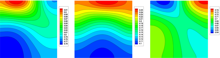
Figure 2.From left to right, there are the contours d11, d12, d22 of the conformation tensor d, respectively

图2. 从左到右，依此是构象张量d的分量d11, d12, d22轮廓图

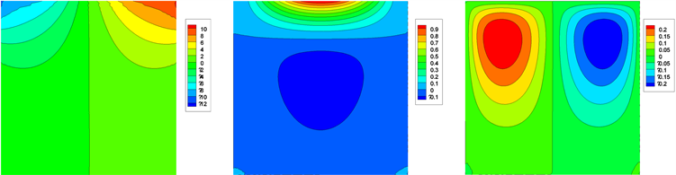
Figure 3. From left to right，there are the contours of pressure p, velocity u1, u2, respectively

图3. 从左到右，依次是压力p，速度u1, u2的轮廓图

5. 小结

本文对扩散Peterlin粘弹性流体提出了时间离散的BDF2压力校正投影方法，避开了速度与压力的不可压缩约束条件。本文证明了该格式的几乎(almost)无条件稳定性。最后通过顶盖驱动方腔流模型检验了该算法的稳定性。下一步我们将对该方法进行误差分析。

基金项目

河南科技大学大学生研究训练计划(SRTP)经费资助：2018188。